Model and Algorithm Evaluation in Supervised Machine Learning

Short Course at CEN 2023 Conference

Max Westphal, Rieke Alpers

Fraunhofer Institute for Digital Medicine MEVIS

2023-09-03

Introduction

Scope

Important topics (50-80%):
- Core concepts
- Performance metrics
- Data splitting
- Statistical analysis

Further considerations (20-50%)
- Practical aspects
- topics not covered in this course…

Learning goal:
- be able to identify common pitfalls for your ML problem…
- … and find suitable (evaluation) solutions.

Housekeeping

Slides & reproducible code
- https://github.com/maxwestphal/evaluation_in_ml_cen_2023
- Attribution-ShareAlike 4.0 International (CC BY-SA 4.0) license

Interactive summaries
- at the end of each section

Questions
- at the end of each section
- online participants: may use the chat

Agenda

Introduction \(\longrightarrow\)
Core Concepts \(\longrightarrow\) \(\longrightarrow\)
Performance metrics \(\longrightarrow\) \(\longrightarrow\)

Break

Data splitting \(\longrightarrow\) \(\longrightarrow\)
Statistical analysis \(\longrightarrow\) \(\longrightarrow\)
Practical aspects \(\longrightarrow\) \(\longrightarrow\)
Wrap-up

Core Concepts

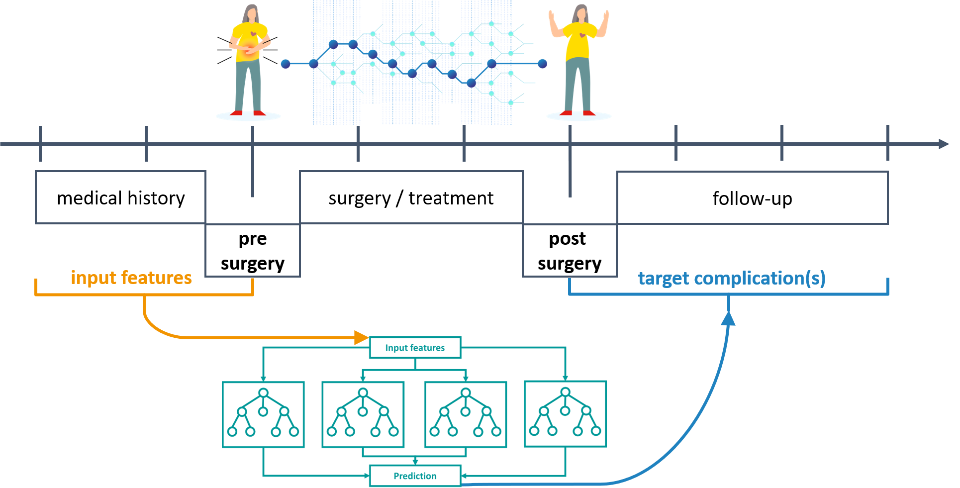
Example project: KIPeriOP

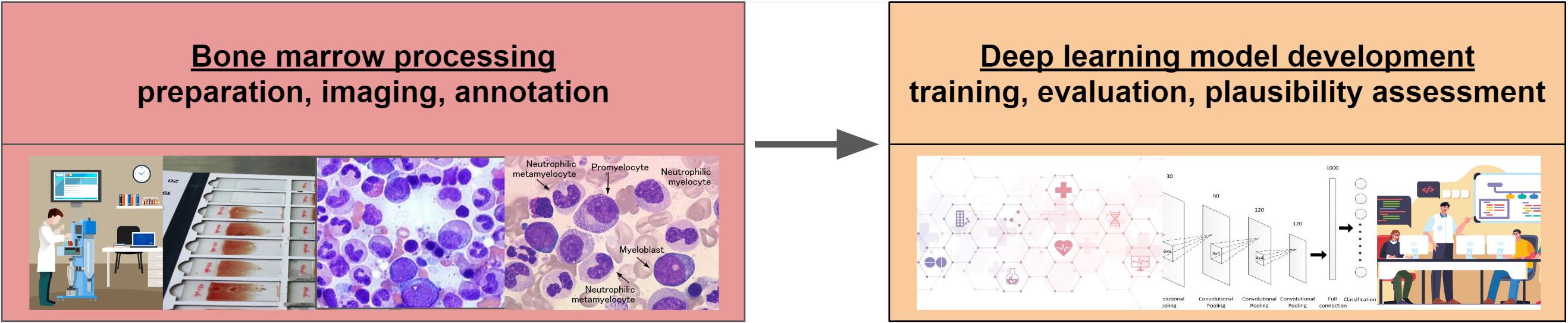
Example project: BMDeep

Example project: CTG

2126 fetal cardiotocograms (CTGs) were automatically processed and the respective diagnostic features measured. The CTGs were also classified by three expert obstetricians and a consensus classification label assigned to each of them. Classification was both with respect to a morphologic pattern (A, B, C. …) and to a fetal state (N, S, P). Therefore the dataset can be used either for 10-class or 3-class experiments

The dataset consists of 2070 observations of 23 features.
In the following, we consider the binary classification task {suspect, pathological} vs. normal

Example project: CTG

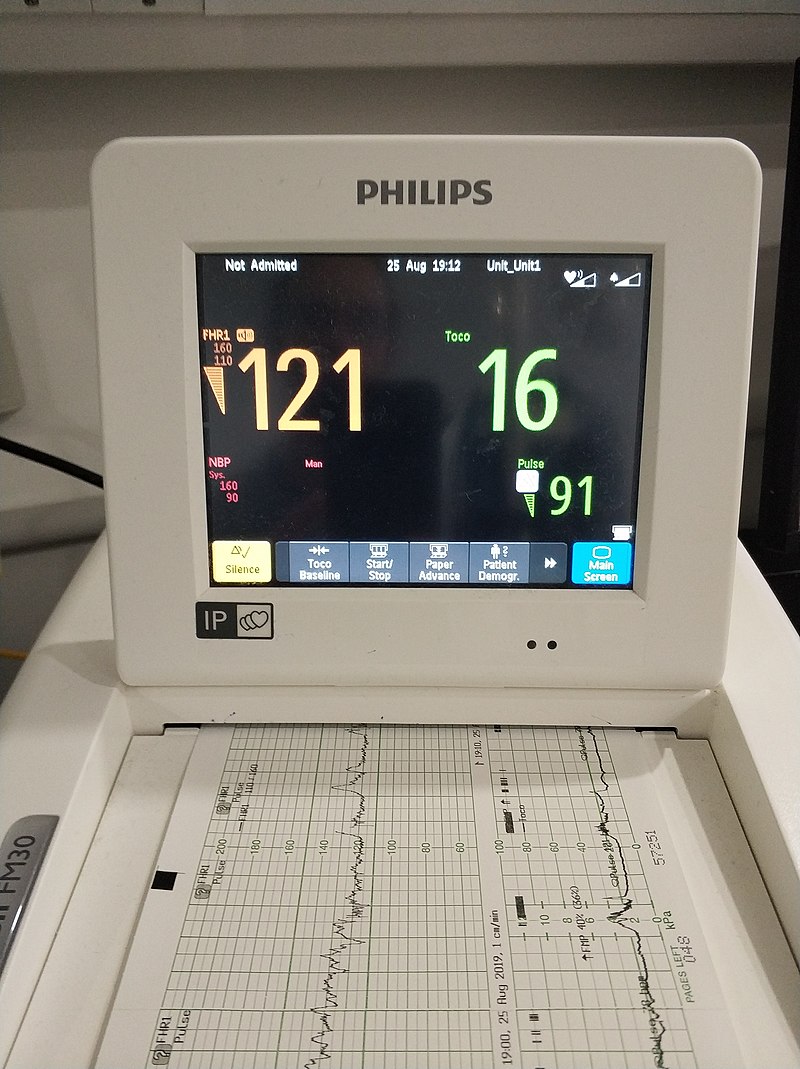
“Cardiotocography (CTG) is a technique used to monitor the fetal heartbeat and uterine contractions during pregnancy and labour. The machine used to perform the monitoring is called a cardiotocograph.”
“CTG monitoring is widely used to assess fetal well-being by identifying babies at risk of hypoxia (lack of oxygen). CTG is mainly used during labour.”
Figure: “The display of a cardiotocograph. The fetal heartbeat is shown in orange, uterine contractions are shown in green, and the small green numbers (lower right) show the mother’s heartbeat.”

Task types in supervised learning

flowchart TB
  ML(Machine learning) --> UL(Unsupervised learning)
  ML --> SL(Supervised learning)
  ML --> RL(Reinforcement learning)
  ML --> dots1(...)
  SL --> BC(binary classification)
  SL --> MCC(multi-class classification)
  SL --> MLC(multi-label classification)
  SL --> TTE(time-to-event analysis)
  SL --> REG(regression)
  SL --> dots2(...)

Focus in this course: binary classification

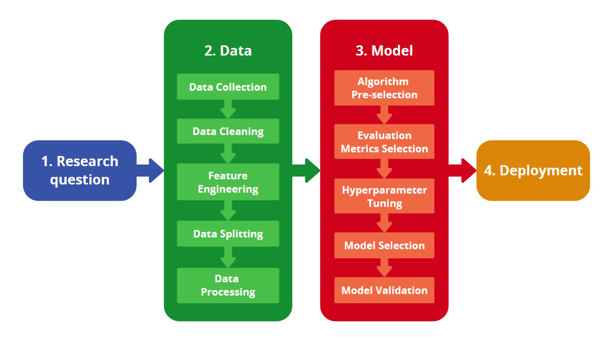
ML workflow

Types of evaluation studies

This course is about evaluation studies assessing (some sort of) performance of prediction models or algorithms
This course is not about assessing the downstream / real-world (clinical) utility

Furthermore, we may distinguish between:
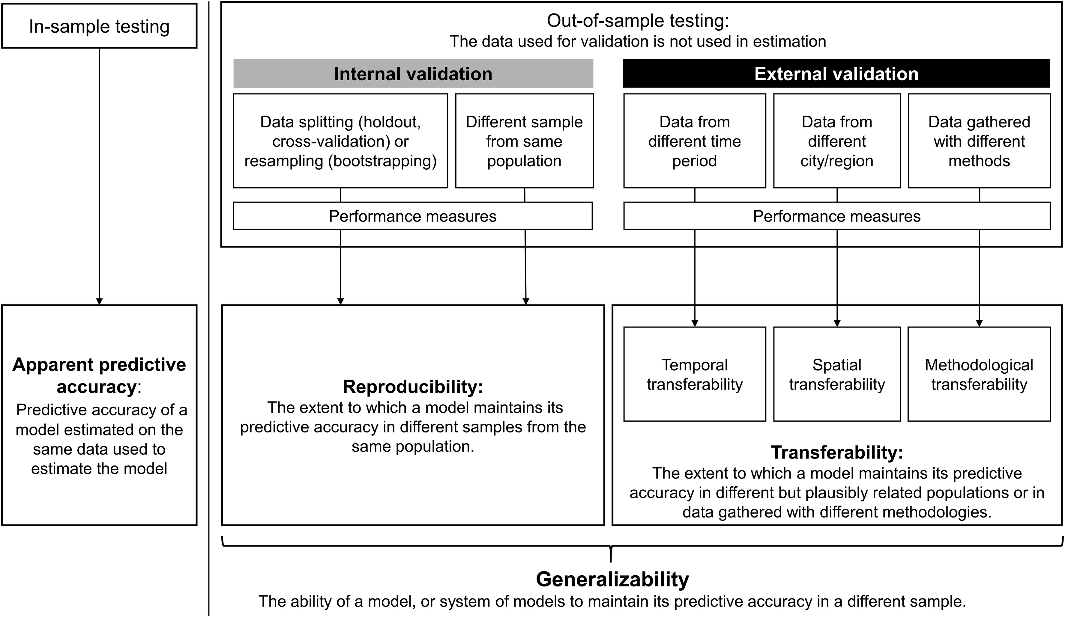
- internal validation: development and evaluation take place in different samples from the same population (in-distrubution)
- external validation: an independent evaluation (different time and/or reseach group)
- internal-external validation: during development, we try to assess the generalizability (transferability) to another context

Applied ML: “standard” pipeline

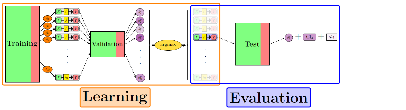
ML terminology is a mess

Training, aka
- Development
- Derivation
- Learning

Tuning, aka
- Validation
- Development

Testing, aka
- Validation
- Evaluation

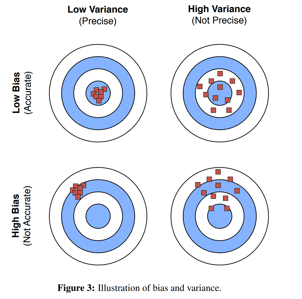
Bias variance trade-off

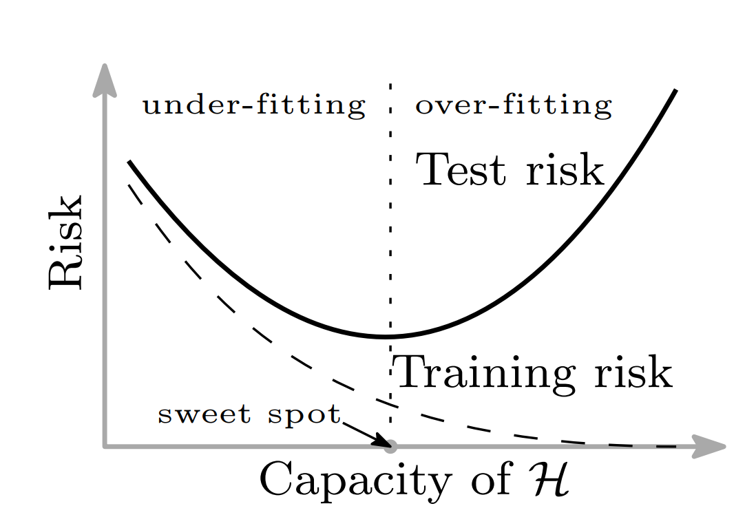
Bias variance trade-off in ML

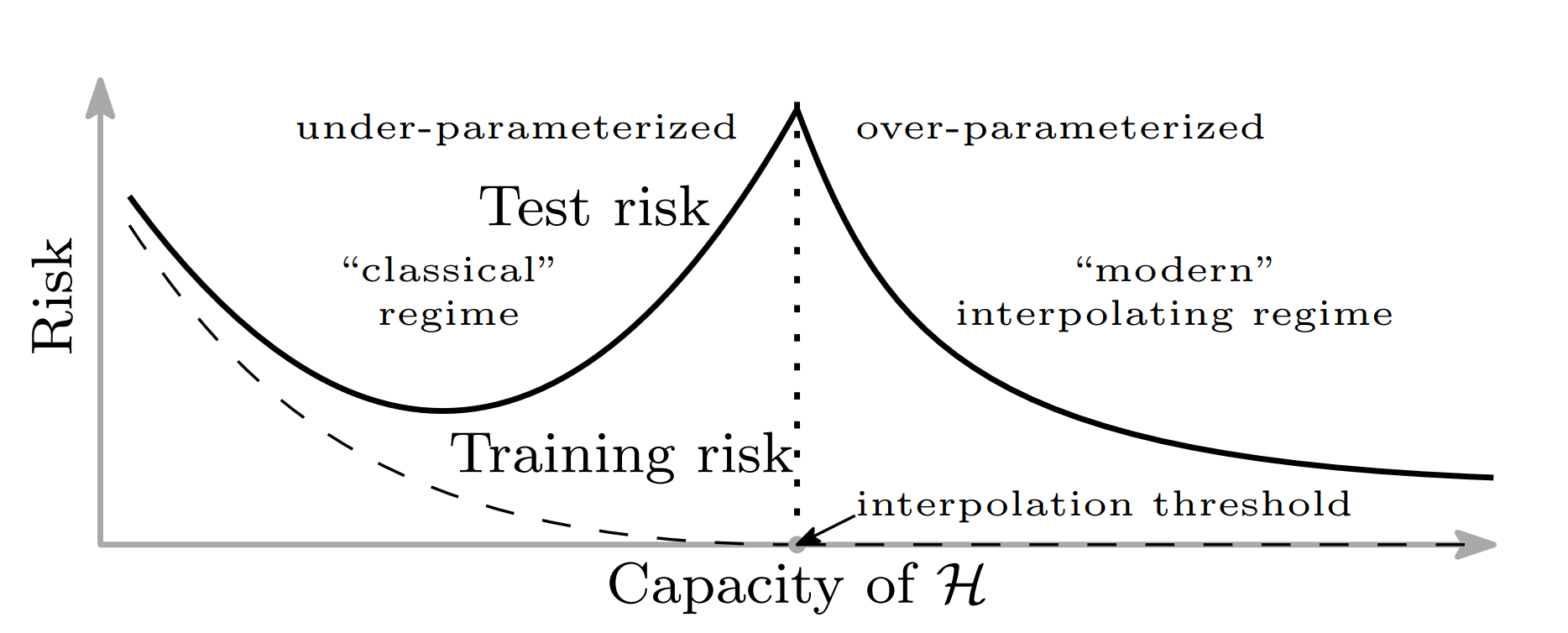
Bias variance trade-off in ML (modern)

Selection-induced bias

Selection-induced bias

No-free-lunch theorem

No single model (architecture) works best in all possible scenarios.

Solutions
- extensive experiments
- inductive bias (prior knowledge)
- a mixture of both

Aleatoric and epistemic uncertainty in machine learning

“Aleatoric (aka statistical) uncertainty refers to the notion of randomness, that is, the variability in the outcome of an experiment which is due to inherently random effects.”
“Epistemic (aka systematic) uncertainty refers to uncertainty caused by a lack of knowledge, i.e., to the epistemic state of the agent.”

Typical ML evaluation pitfalls

Typical ML pitfalls

Interactive summary

Q1: What is NOT a typical pitfall in ML evaluation studies?

data augmentation before data splitting
ignoring temporal dependencies
only evaluate each model once
combined model tuning and evaluation on the test data

Q1: What is NOT a typical pitfall in ML evaluation studies?

data augmentation before data splitting
ignoring temporal dependencies
only evaluate each model once
combined model tuning and evaluation on the test data

Q2: Three datasets are needed in the standard ML pipeline to counter …

overfitting and underfitting
overfitting and selection-induced bias
underfitting and selection-induced bias
overfitting, underfitting and selection-induced bias

Q2: Three datasets are needed in the standard ML pipeline to counter …

overfitting and underfitting
overfitting and selection-induced bias
underfitting and selection-induced bias
overfitting, underfitting and selection-induced bias

Q3: What type of validation does NOT exist?

external-internal
internal-external
external
internal

Q3: What type of validation does NOT exist?

external-internal
internal-external
external
internal

Q4: What is NOT a valid ML task?

multil-label classification
time-to-event analysis
binary classification
multi-class regression

Q4: What is NOT a valid ML task?

multil-label classification
time-to-event analysis
binary classification
multi-class regression

Q5: When comparing multiple models on the same dataset, the severity of selection-induced bias…

decreases with model similarity
decreases with the number of models
decreases with spread of true performances
increases with spread of true performances

Q5: When comparing multiple models on the same dataset, the severity of selection-induced bias…

decreases with model similarity
decreases with the number of models
decreases with spread of true performances
increases with spread of true performances

Questions

Performance metrics

Performance dimensions

Discrimintation: can the model distinguish between the target classes?
Calibration: are probability prediction accurate?
Fairness: is discrimination similar in important subgroups?

Uncertainty quantification: how good is the coverage of prediction intervals?
Explainability: usually assessed in user studies…

Metric choice

A deliberate metric choice is very important for a successful ML project.
- a sensible metric supports/guides development
- an unreasonable metric hinders development

What is an optimal solution worth, if it is optimal w.r.t. to a suboptimal metric?

Finding an adequate metric can be time consuming
- should be done early on (before any developments)
- should be based on discussion with important stakeholders (e.g. potential users)

“Standard” / “default” metrics in the field:
- usually a good idea to report as well (secondary)
- often not sufficient as primary / sole metric

Multiple interesting metrics?
- Development usually facilitated if there is a clear decision rule how to rank models (e.g. primary metric)

Metrics: R packages

Metrics: https://CRAN.R-project.org/package=Metrics (2018-07-09)
ModelMetrics: https://CRAN.R-project.org/package=ModelMetrics ( 2020-03-17)
metrica: https://CRAN.R-project.org/package=metrica (2023-04-14)
SurvMetrics: https://CRAN.R-project.org/package=SurvMetrics (2022-09-03)
MetricsWeighted: https://CRAN.R-project.org/package=Metrics (2023-06-05)

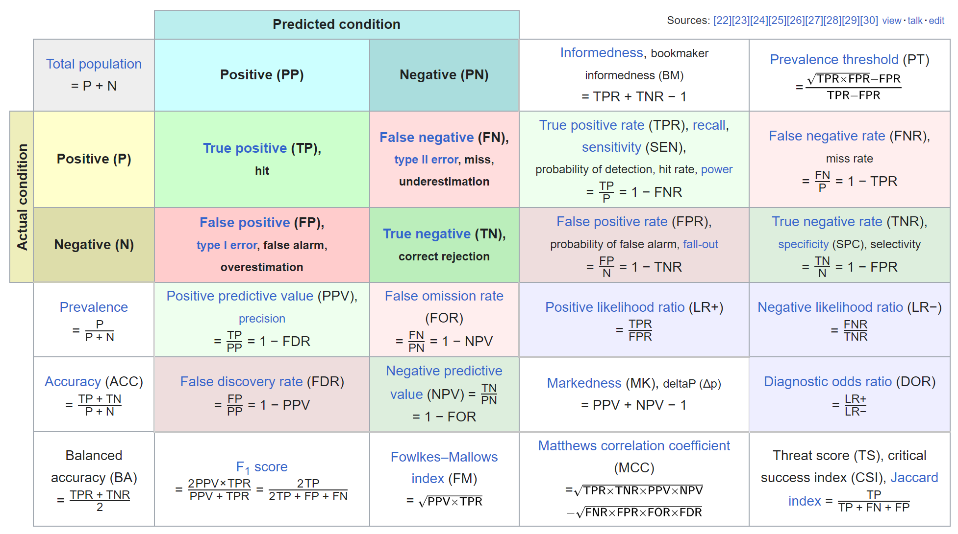
Binary classification: confusion matrix

Evaluation data for CTG example (train-tune-test)

dim(data_eval_ttt_1)

[1] 412   5

head(data_eval_ttt_1)

  row_ids  truth response prob.suspect prob.normal
1       3 normal   normal   0.42001441   0.5799856
2      19 normal   normal   0.00000000   1.0000000
3      28 normal   normal   0.03574335   0.9642566
4      31 normal   normal   0.04821049   0.9517895
5      47 normal   normal   0.00000000   1.0000000
6      48 normal   normal   0.00000000   1.0000000

mean((data_eval_ttt_1$response == "suspect") == 
       (data_eval_ttt_1$prob.suspect > 0.5))

[1] 1

Binary classification: confusion matrix

caret::confusionMatrix(reference = data_eval_ttt_1$truth,
                       data = data_eval_ttt_1$response,
                       positive = "suspect")

Confusion Matrix and Statistics

          Reference
Prediction suspect normal
   suspect      75      3
   normal       15    319
                                          
               Accuracy : 0.9563          
                 95% CI : (0.9318, 0.9739)
    No Information Rate : 0.7816          
    P-Value [Acc > NIR] : < 2.2e-16       
                                          
                  Kappa : 0.8656          
                                          
 Mcnemar's Test P-Value : 0.009522        
                                          
            Sensitivity : 0.8333          
            Specificity : 0.9907          
         Pos Pred Value : 0.9615          
         Neg Pred Value : 0.9551          
             Prevalence : 0.2184          
         Detection Rate : 0.1820          
   Detection Prevalence : 0.1893          
      Balanced Accuracy : 0.9120          
                                          
       'Positive' Class : suspect

Binary classification: discrimination metrics

Accuracy: Probability of correct classification (actual \(=\) predicted)
Sensitivity: Accuracy in positive class (cases, diseased, 1, TRUE)
Specificity: Accuracy in negative class (controls, healthy, 0, FALSE)
PPV: Accuracy in positive predictions
NPV: Accuracy in negative predictions
Balanced accuracy: Average of sensitivity and specificiy

Binary classification: weighted accuracy

a <- data_eval_ttt_1$truth == "suspect"
p <- data_eval_ttt_1$response == "suspect"
Metrics::accuracy(actual = a, predicted = p)

[1] 0.9563107

m <- 5 # sensitvity to be weighted m times higher compared to specificity
w <- m / (1+m) # weight for sensitivity

w*ModelMetrics::sensitivity(a, p) + 
  (1-w)*ModelMetrics::specificity(a, p)

[1] 0.8595583

Binary classification: Risk prediction

Binary classifier which not only predict the target variable (TRUE vs. FALSE), but also a probability of an event (TRUE), may also be called risk prediction models
Often fundamental requirement in clinical predictive modelling
As domain experts shall usually be supported (not replaced) by ML models / algorithms, a predicted risk can be much more informative and interpretable compared to a model only capable of predicting class labels

Receiver operating characteristic (ROC)

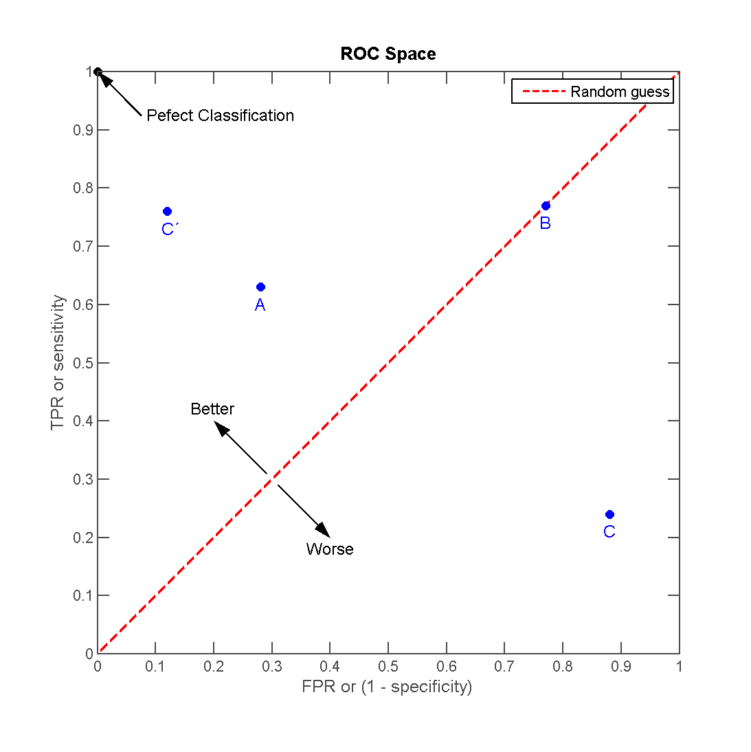
Receiver operating characteristic (ROC)

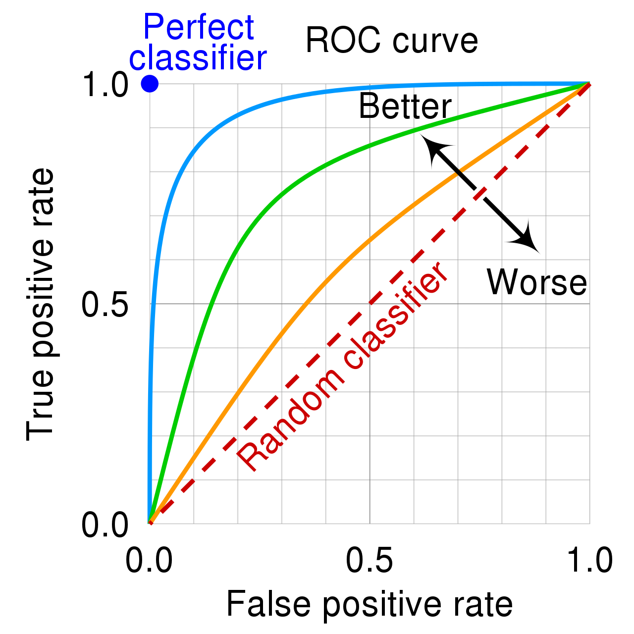
Receiver operating characteristic (ROC)

rocc <- pROC::roc(data_eval_ttt_1, response="truth", predictor="prob.suspect", levels=c("normal", "suspect"))

plot(rocc)

Binary classification: Area under the curve (AUC)

Area under the (ROC) curve (also “c-statistic”, “concordance statistic”)
- Interpretation:
- Partial AUC: restrict specificity range
- Many different implementations (smoothed, with CI)

Binary classification: Area under the curve (AUC)

pROC::auc(rocc)

Area under the curve: 0.9831

pROC::auc(rocc, partial.auc=c(0.5, 1), partial.auc.correct=TRUE)

Corrected partial area under the curve (specificity 1-0.5): 0.9775

Binary classification: calibration plot

caret::calibration(truth ~ prob.suspect, data=data_eval_ttt_1) %>% plot()

Binary classification: calibration plot

df <- data_eval_ttt_1 %>% mutate(truth = truth=="suspect")
predtools::calibration_plot(df, obs="truth", pred="prob.suspect")

$calibration_plot

Binary classification: calibration plot

CalibratR::reliability_diagramm(actual = data_eval_ttt_1$truth == "suspect",
                                predicted = data_eval_ttt_1$prob.suspect)$diagram_plot

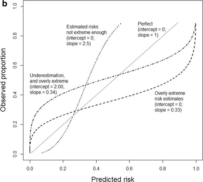
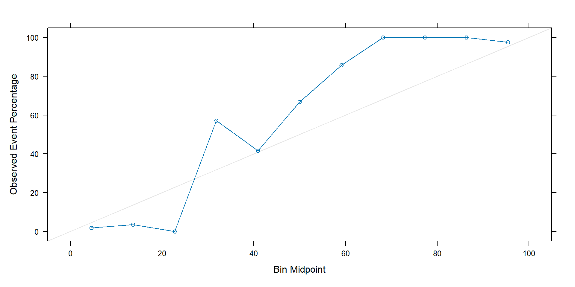
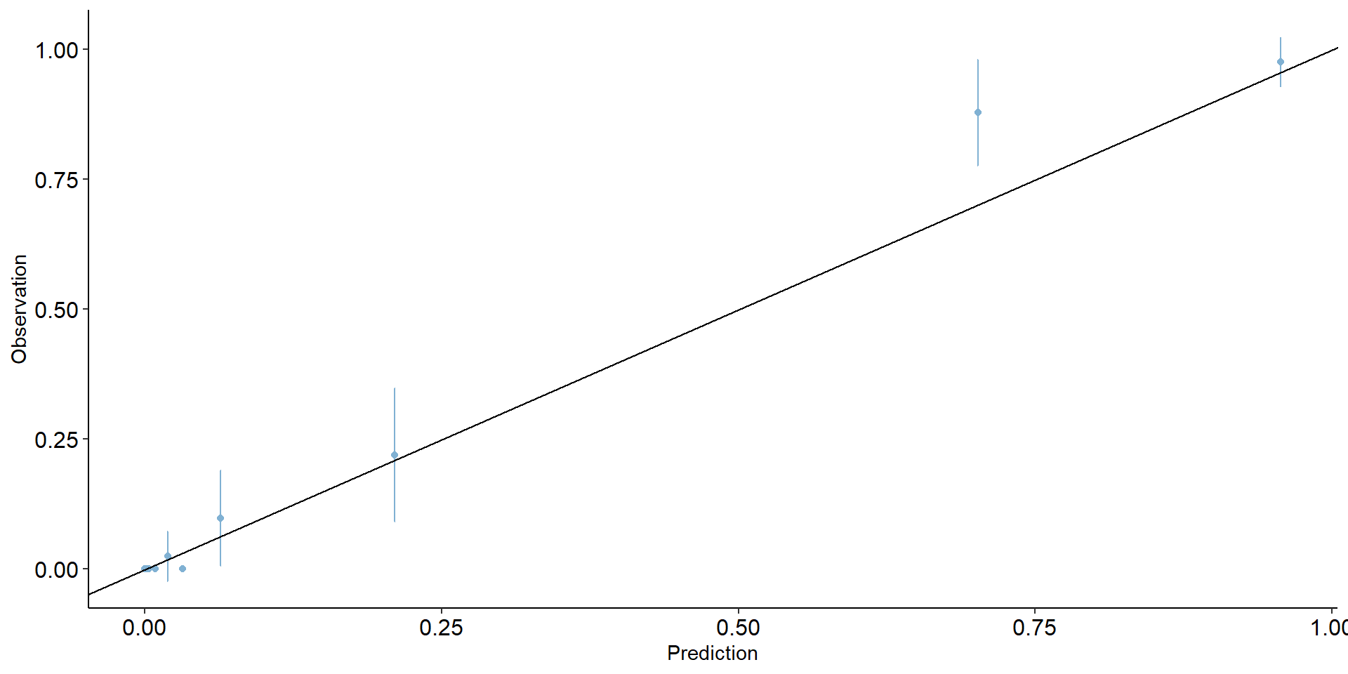
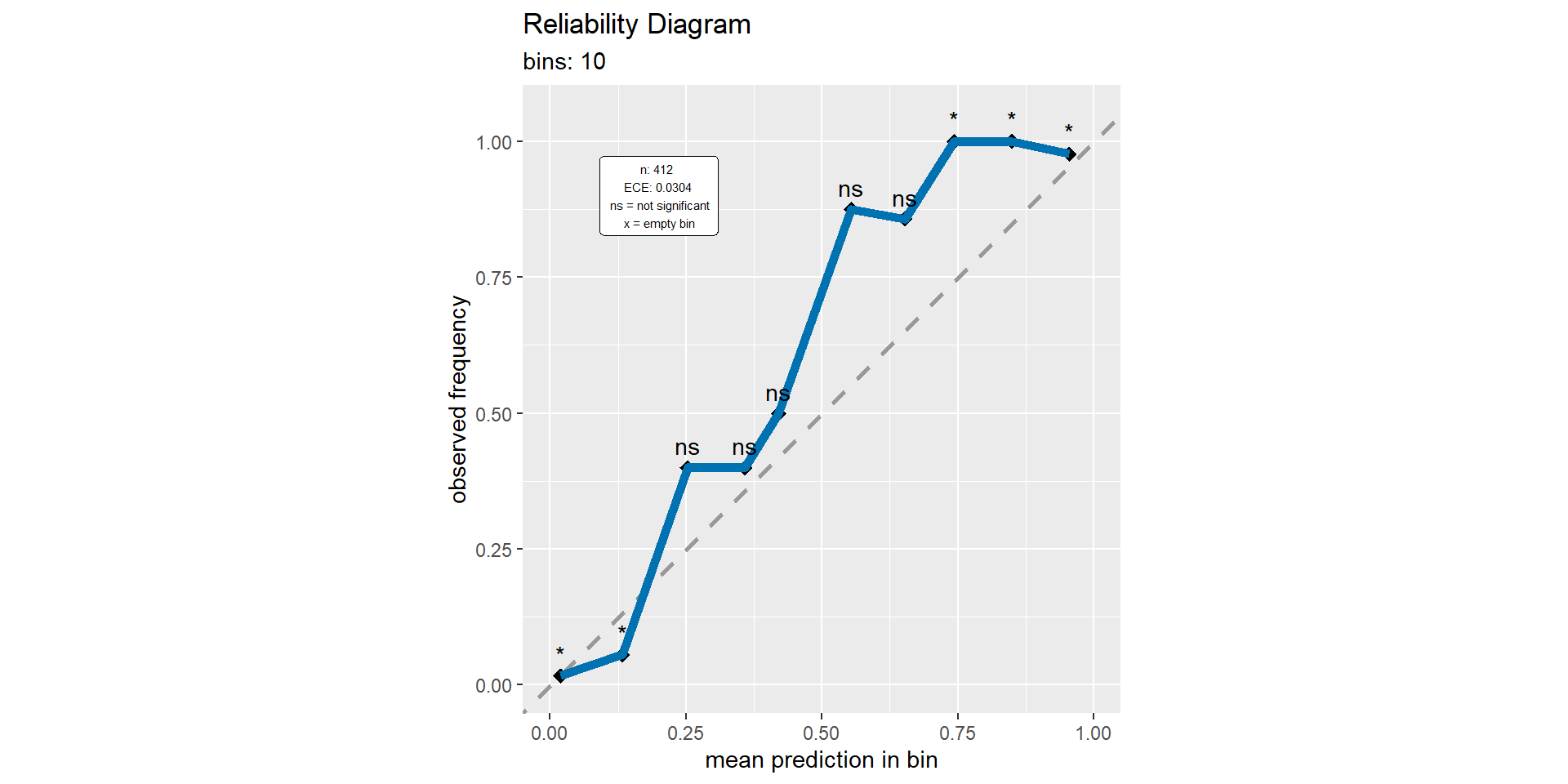
Binary classification: calibration metrics

Expected calibration error (ECE)
Maximum calibration error (MCE)
Root mean squared error (from diagonal) (RSME)

Calibration intercept (calibration-in-the-large)
Calibration slope

Binary classification: calibration metrics

a <- data_eval_ttt_1$truth == "suspect"
p <- data_eval_ttt_1$prob.suspect

CalibratR::getECE(actual = a, predicted=p, n_bins=10)

[1] 0.02858147

CalibratR::getECE(actual = a, predicted=p, n_bins=20)

[1] 0.03823656

Binary classification: calibration metrics

CalibratR::getMCE(actual = a, predicted=p, n_bins=10)

[1] 0.01754832

CalibratR::getMCE(actual = a, predicted=p, n_bins=20)

[1] 0.01209066

Calibration slope and intercept

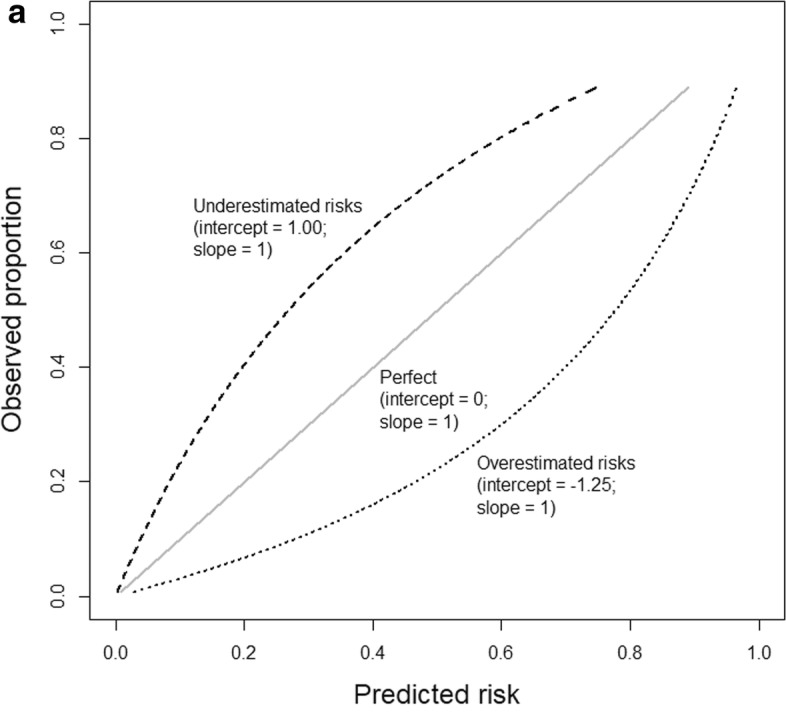
Calibration slope and intercept

Binary classification: fairness - overview

Predictive rate parity
False positive rate parity
False negative rate parity
Accuracy parity
Negative predictive value parity
Specificity parity
ROC AUC parity
…

Multi-class classification: Confusion matrix

set.seed(123)
a <- rep(letters[1:5], times= (1:5)*20)
p <- sample(a, length(a))

caret::confusionMatrix(data = as.factor(p), reference=as.factor(a))

Confusion Matrix and Statistics

          Reference
Prediction  a  b  c  d  e
         a  2  4  2  5  7
         b  1  7  9 11 12
         c  4  9 14 15 18
         d  5  6 20 22 27
         e  8 14 15 27 36

Overall Statistics
                                         
               Accuracy : 0.27           
                 95% CI : (0.2206, 0.324)
    No Information Rate : 0.3333         
    P-Value [Acc > NIR] : 0.9924         
                                         
                  Kappa : 0.0338         
                                         
 Mcnemar's Test P-Value : 0.8813         

Statistics by Class:

                     Class: a Class: b Class: c Class: d Class: e
Sensitivity          0.100000  0.17500  0.23333  0.27500   0.3600
Specificity          0.935714  0.87308  0.80833  0.73636   0.6800
Pos Pred Value       0.100000  0.17500  0.23333  0.27500   0.3600
Neg Pred Value       0.935714  0.87308  0.80833  0.73636   0.6800
Prevalence           0.066667  0.13333  0.20000  0.26667   0.3333
Detection Rate       0.006667  0.02333  0.04667  0.07333   0.1200
Detection Prevalence 0.066667  0.13333  0.20000  0.26667   0.3333
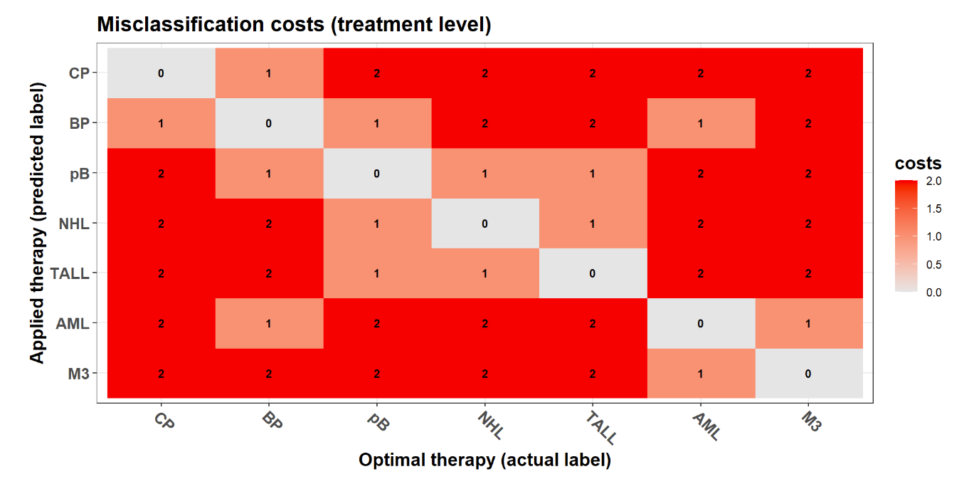
Balanced Accuracy    0.517857  0.52404  0.52083  0.50568   0.5200

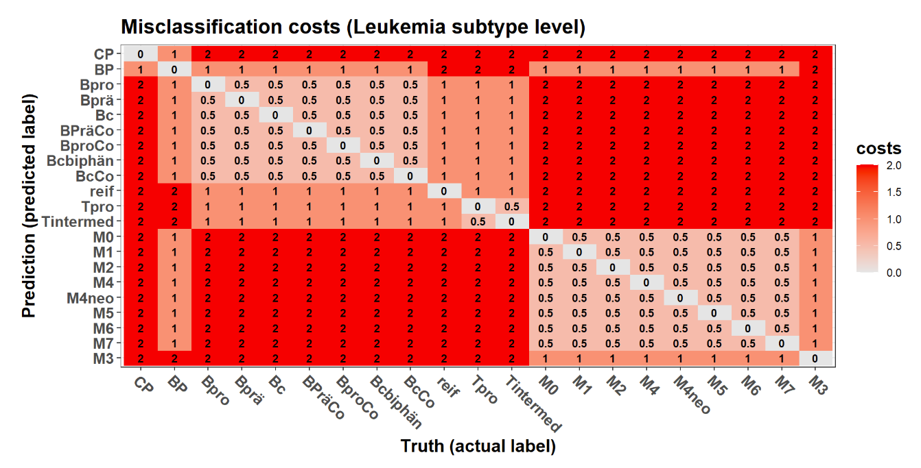
Multi-class classification: cost-sensitive metrics (BMDeep)

Regression: loss functions

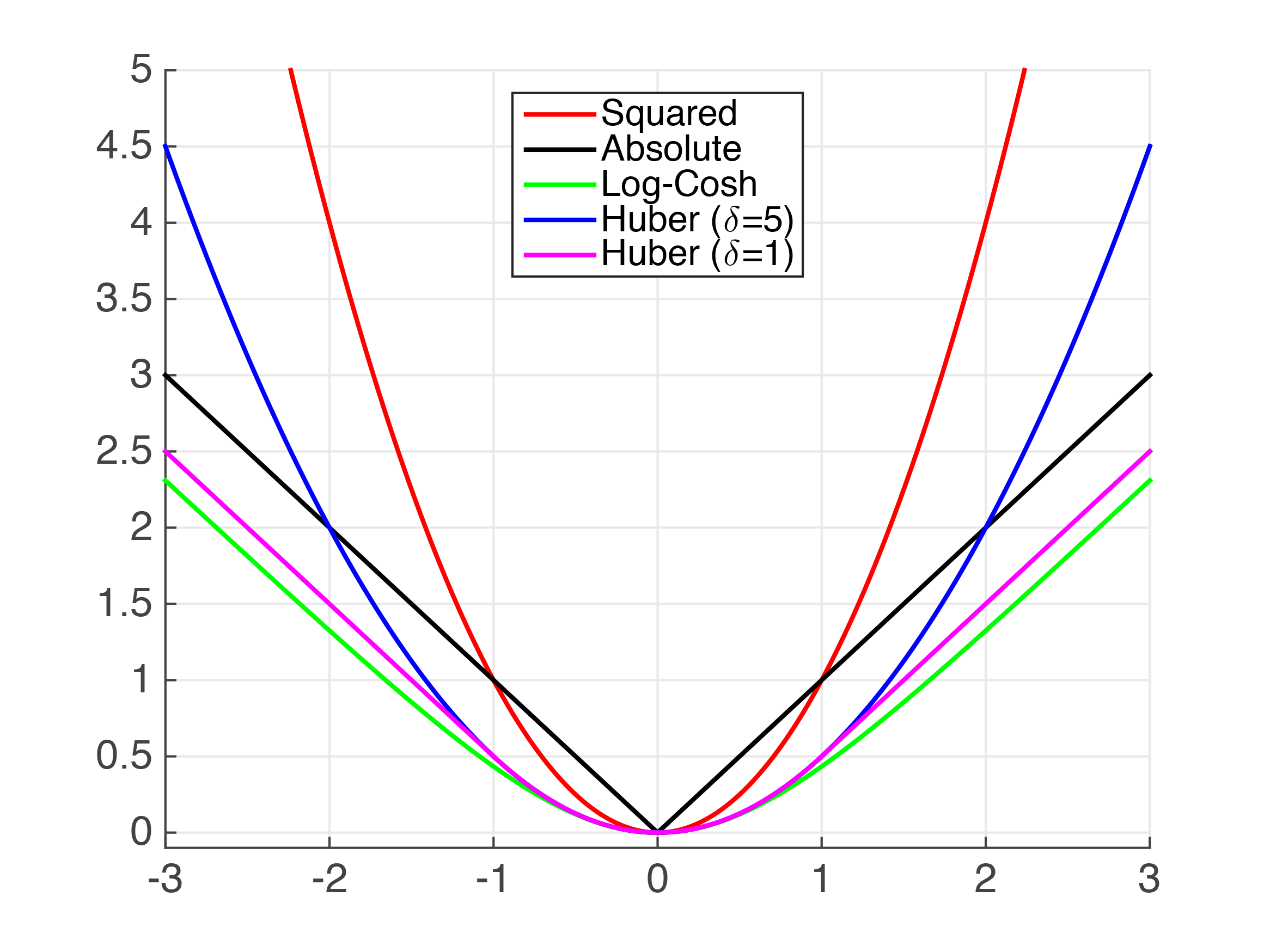
Regression: loss functions

Symmetric loss functions used to define frequently used regression performance metrics, e.g.
- mean squared error
- mean absolute error
For some regression tasks, custom performance metrics (based on asymmetric loss functions) may be more suitable
- for details, see references below

Survival analysis: overview

Mean absolute error (and other regression metrics)
- Not recommended as censoring is ignored
Concordance index/measure
- probability that of a randomly selected pair of patients , the patient with the shorter survival time has the higher predicted risk.
- most freuqently used
- several versions do exist
(Integrated) Brier score
Calibration slope

Metric choice

A deliberate metric choice is very important for a successful ML project.
- a sensible metric supports/guides development
- an unreasonable metric hinders development

What is an optimal solution worth, if it is optimal w.r.t. to a suboptimal metric?

Finding an adequate metric can be time consuming
- should be done early on (before any developments)
- should be based on discussion with important stakeholders (e.g. potential users)

“Standard” / “default” metrics in the field:
- usually a good idea to report as well (secondary)
- often not sufficient as primary / sole metric

Multiple interesting metrics?
- Development usually facilitated if there is a clear decision rule how to rank models (e.g. primary metric)

Interactive summary

Q1: What is displayed in the confusion matrix?

actual labels vs. predicted labels
predicted labels vs. estimated probabilities
actual labels vs. observed frequencies
observed frequencies vs. estimated probabilities

Q1: What is displayed in the confusion matrix?

actual labels vs. predicted labels
predicted labels vs. estimated probabilities
actual labels vs. observed frequencies
observed frequencies vs. estimated probabilities

Q2: Which of the following metrics is NOT applicable to all binary classifiers?

specificty
accuracy
positive predictive value
area under the curve

Q2: Which of the following metrics is NOT applicable to all binary classifiers?

specificty
accuracy
positive predictive value
area under the curve

Q3: Calibration assesses …

predicted probabilities relative to observed class labels
predicted probabilities relative to observed class frequencies
predicted class labels relative to the majority class
predicted class labels relative to the minority class

Q3: Calibration assesses …

predicted probabilities relative to observed class labels
predicted probabilities relative to observed class frequencies
predicted class labels relative to the majority class
predicted class labels relative to the minority class

Q4: Which of the following statements is true?

only sensitivty OR specifity should be considered, not both
overall accuracy is independed of class prevalences
balanced accuracy can be calculated from the confusing matrix
balanced accuracy can be calculated from the confusion matrix

Q4: Which of the following statements is true?

only sensitivty OR specifity should be considered, not both
overall accuracy is independed of class prevalences
balanced accuracy can be calculated from the confusing matrix
balanced accuracy can be calculated from the confusion matrix

Q5: Which metrics can be used for the same ML task?

balanced accuracy and mean squared error
mean squared error and maximum calibration error
area under the curve and maximum calibration error
mean squared error and area under the curve

Q5: Which metrics can be used for the same ML task?

balanced accuracy and mean squared error
mean squared error and maximum calibration error
area under the curve and maximum calibration error
mean squared error and area under the curve

Questions

Break

Data splitting

Motivation: overfitting

Motivation: selection-induced bias

Overview of approaches

Train-tune-test split
Cross-validation (CV)
Bootstrapping

Stratified splitting
Grouped (blocked) splitting

Nested splitting (nested CV)

Special variants (e.g. for time-series data)

The “default” train-tune-test split

The “default” train-tune-test split

(Was used so far in the previous section)
Simple to implement
Low computational effort
Simple statistical inference
Target: conditional performance, either of…
- model trained on “train” dataset
- model trained on “train” & “tune” datasets combined

Cross-validation (+ independent test set)

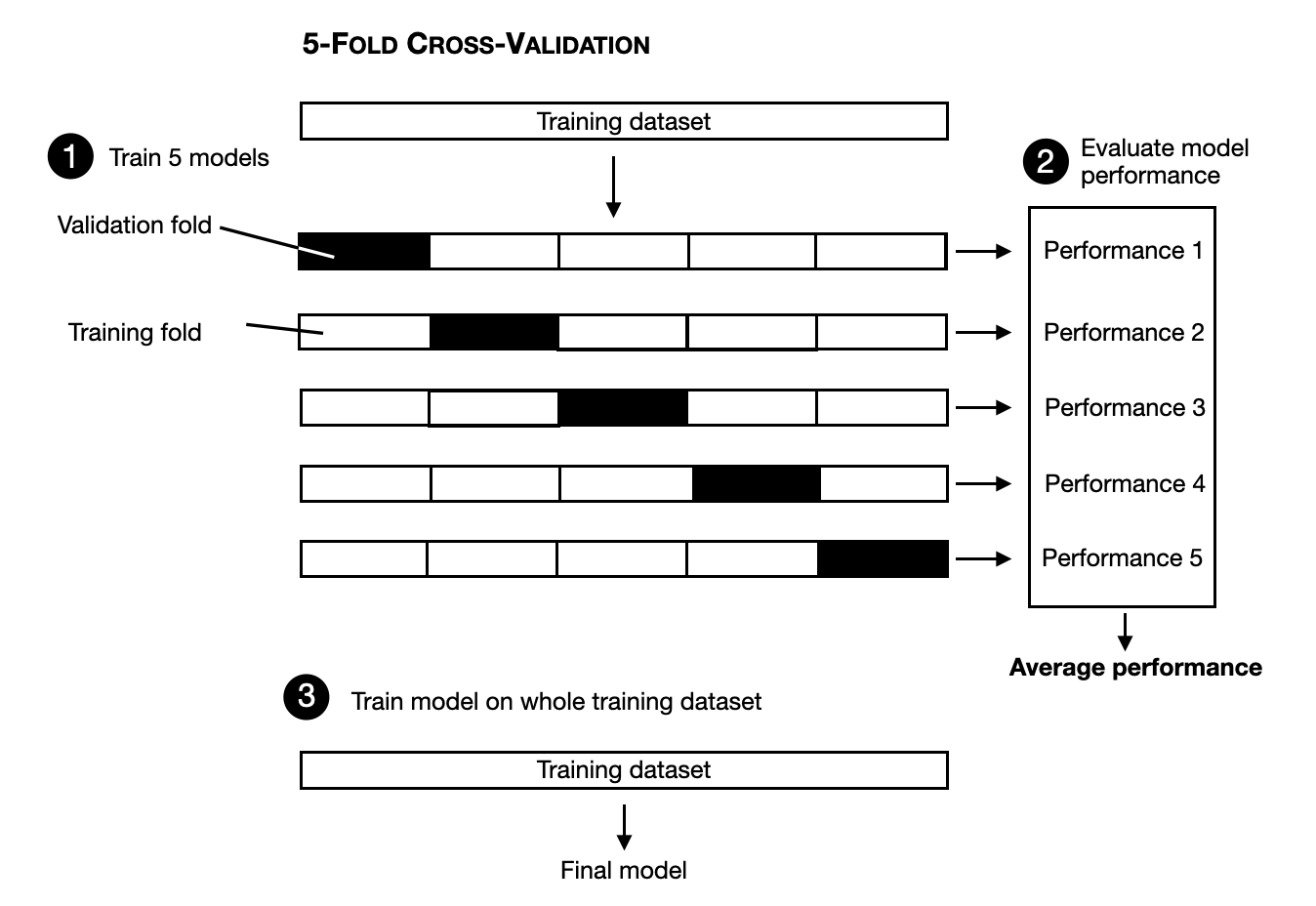
Cross-validation (+ independent test set)

Cross-validation (cross-tuning):
- unconditional performance assessed
- increased computational burden (by number of folds \(K\))
- reduces danger of bad model selection for small samples

Is the independent test set really required?
It depends:
- Only model comparison needed: no
- Only performance assessment: no
- Both needed: yes, as (CV based) performance estimate of (CV) selected model can still be biased

Solution: Nested cross-validation

Nested cross-validation

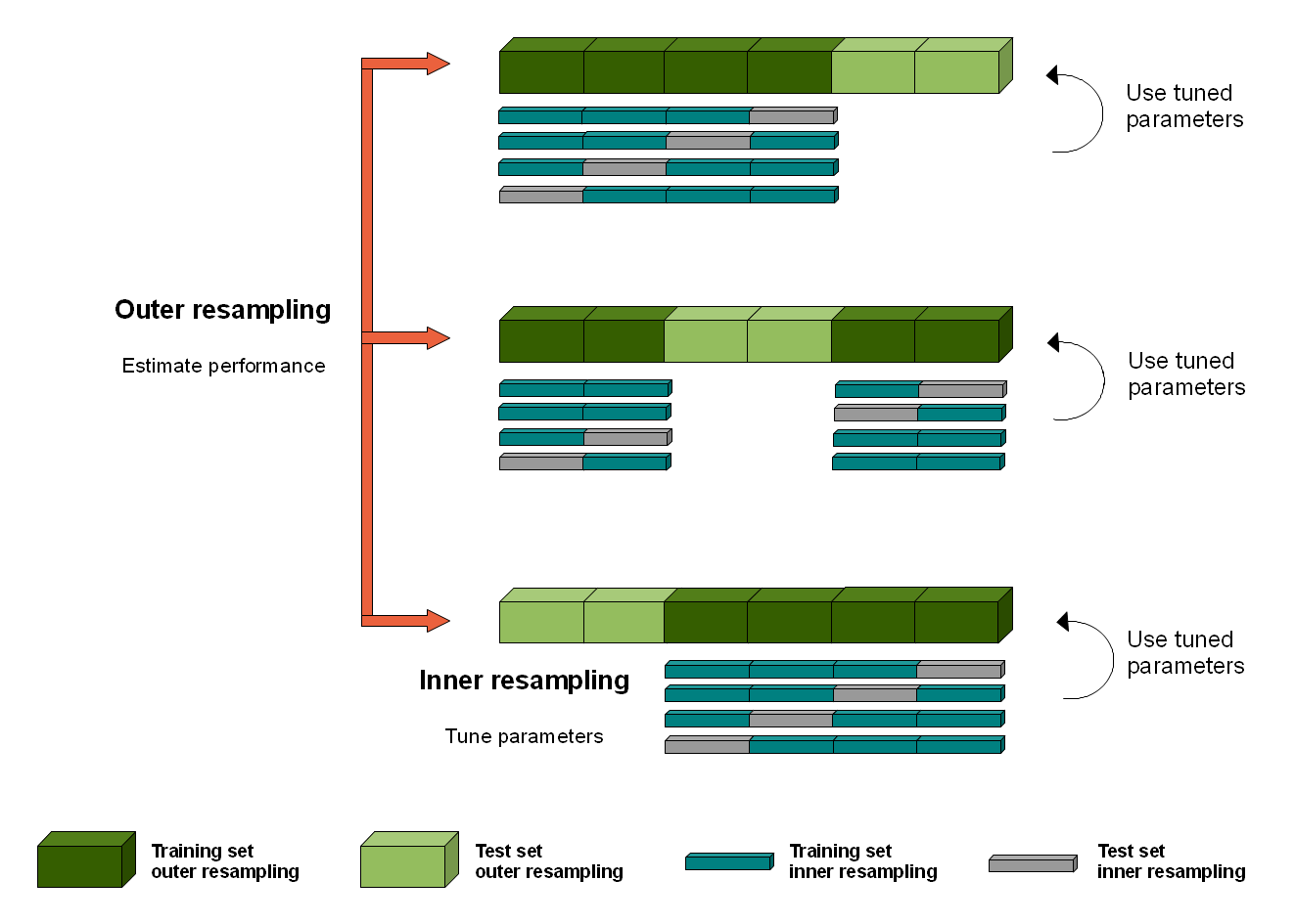
Computational complexity

Train-tune-test: \(1\)
K-fold CV: \(K\) (number of folds)
Nested CV: \(K_{\text{inner}}\ \cdot K_{\text{outer}}\)
Bootstrap: \(B\) (number of bootstrap repetitions)
R-repeated K-fold CV: \(R \cdot K\)
Leave-one-out CV: \(n_{\text{obs}}\) (number of observations)

General recommendations

Trade off of between complexity (implementation, computation, analysis) and sample efficiency

Large n: train/tune/test
- simple (implementation, computation, analysis)

Small n: (nested) CV
- higher compute due to repeated sampling/training

Optimal splitting (number of folds, ratio)
- no general accepted solution
- simulation…
- power calculation can guide minimal test set size

Splitting variants

Stratification: should the distribution of certain variables be (approximately) equal in all datasets?
- In particular relevant for the outcome variable (classification)
- No/low costs, medium/high reward

Grouping (also: blocking): Very relevant for hierarchical data
Relevant question: What is the observational unit of your study?
- a (e.g. bone marrow) cell
- an image / a BM smear (= a collection of cells)
- a patient (= potentially multiple BM smears)
If a lower hierarchy level is chosen, then splitting should be grouped by patient

There is more to it…

Almost all data splitting techniques so far relied on random partitioning or sub-sampling
For non-IID observations, e.g. time-series data, special data splitting methods are required (Schnaubelt, 2019)
Question: What quantity are we really interested in?
Observation: “generalization performance” is usually not defined very precisely in ML

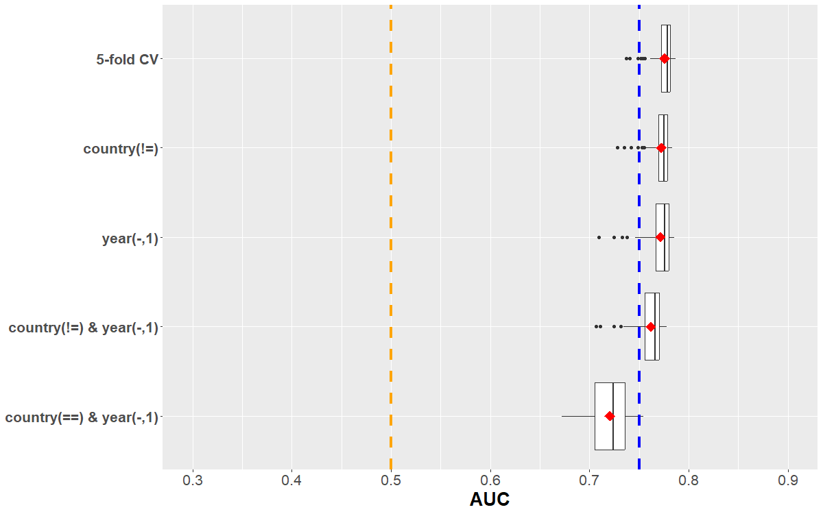
Generalizability vs. transferability

Estimand framework

Interactive summary

Q1: What is a commonly used data splitting technique?

train-validation-test
train-tune-test
tune-validation
cross-validation

Q1: What is a commonly used data splitting technique?

train-validation-test
train-tune-test
tune-validation
cross-validation

Q2: Which data splitting techniques are rarely used due to very high computational effort for model training?

5-fold cross-validation and the bootstrap
the bootstrap and leave-one-out cross-validation
100-fold cross-validation and the train-tune-test split
the bootstrap and the train-tune-test split

Q2: Which data splitting techniques are rarely used due to very high computational effort for model training?

5-fold cross-validation and the bootstrap
the bootstrap and leave-one-out cross-validation
100-fold cross-validation and the train-tune-test split
the bootstrap and the train-tune-test split

Q3: For large datasets, the classical “train-tune-test” split can be recommended due to…

simple statistical analysis
utilization of all observations for testing
being the default method in many packages
minimal computational effort

Q3: For large datasets, the classical “train-tune-test” split can be recommended due to…

simple statistical analysis
utilization of all observations for testing
being the default method in many packages
minimal computational effort

Q4: For small datasets, …

a proper model comparison and evaluation is usually simpler
nested data splitting techniques have increased relevance
no data should be wasted for method evaluation
the importance of power estimation is increased

Q4: For small datasets, …

a proper model comparison and evaluation is usually simpler
nested data splitting techniques have increased relevance
no data should be wasted for method evaluation
the importance of power estimation is increased

Q5: Which of the following statements is true?

Stratification is required for hierarchical data structures
Grouping is required for hierarchical data structures
Stratification is required to retain the class distribution
Grouping is required to retain the class distribution

Q5: Which of the following statements is true?

Stratification is required for hierarchical data structures
Grouping is required for hierarchical data structures
Stratification is required to retain the class distribution
Grouping is required to retain the class distribution

Questions

Statistical analysis

Goals of statistical inference

Estimation
Uncertainty quantification
- standard error
- confidence interval
Decision making
- hypothesis testing

Overview

Classical (frequentist) inference
Nonparametric methods
- bootstrap
- hierarchical bootstrap
Complex procedures
- mixed models
- Bayesian inference

Choice of comparator

none (descriptive analysis)

fixed performance threshold \(\vartheta_0 = 0.8\)

another (established) prediction model: \(\vartheta_0 = \vartheta(\hat{f}_0)\)
- same test data
- paired comparison (!)

Evaluation data: train-tune-test (model comparison)

Scenario: a random forest model was (hyperparameter) tuned on the train/tune data. The best/final model (w.r.t. tuning AUC) shall now be compared against an established elastic net model.
Null hypothesis: \(\vartheta^\text{ranger}_* = \vartheta^\text{glmnet}_0\) (no difference in performance)

head(data_eval_ttt_2)

   row_ids  truth response_glmnet prob.suspect_glmnet prob.normal_glmnet
1:       3 normal          normal        2.663412e-02          0.9733659
2:      19 normal          normal        7.350806e-03          0.9926492
3:      28 normal          normal        2.207659e-04          0.9997792
4:      31 normal          normal        2.015005e-05          0.9999798
5:      47 normal          normal        1.646076e-04          0.9998354
6:      48 normal          normal        4.657763e-04          0.9995342
   response_ranger prob.suspect_ranger prob.normal_ranger
1:          normal          0.42001441          0.5799856
2:          normal          0.00000000          1.0000000
3:          normal          0.03574335          0.9642566
4:          normal          0.04821049          0.9517895
5:          normal          0.00000000          1.0000000
6:          normal          0.00000000          1.0000000

Data preparation

actual <- data_eval_ttt_2$truth
actual_01 <- (actual == "suspect") %>% as.numeric()

pred_glmnet <- data_eval_ttt_2$response_glmnet 
pred_glmnet_01 <- (pred_glmnet== "suspect") %>% as.numeric()
correct_glmnet_01 <- (pred_glmnet_01 == actual_01) %>% as.numeric()

pred_ranger <- data_eval_ttt_2$response_ranger 
pred_ranger_01 <- (pred_ranger== "suspect") %>% as.numeric()
correct_ranger_01 <- (pred_ranger_01 == actual_01) %>% as.numeric()

Model 1: elastic net (glmnet)

caret::confusionMatrix(data = pred_glmnet, reference = actual)

Confusion Matrix and Statistics

          Reference
Prediction suspect normal
   suspect      69      8
   normal       21    314
                                          
               Accuracy : 0.9296          
                 95% CI : (0.9005, 0.9524)
    No Information Rate : 0.7816          
    P-Value [Acc > NIR] : 2.668e-16       
                                          
                  Kappa : 0.7825          
                                          
 Mcnemar's Test P-Value : 0.02586         
                                          
            Sensitivity : 0.7667          
            Specificity : 0.9752          
         Pos Pred Value : 0.8961          
         Neg Pred Value : 0.9373          
             Prevalence : 0.2184          
         Detection Rate : 0.1675          
   Detection Prevalence : 0.1869          
      Balanced Accuracy : 0.8709          
                                          
       'Positive' Class : suspect

Model 2: random forest (ranger)

caret::confusionMatrix(data = pred_ranger, reference = actual)

Confusion Matrix and Statistics

          Reference
Prediction suspect normal
   suspect      75      3
   normal       15    319
                                          
               Accuracy : 0.9563          
                 95% CI : (0.9318, 0.9739)
    No Information Rate : 0.7816          
    P-Value [Acc > NIR] : < 2.2e-16       
                                          
                  Kappa : 0.8656          
                                          
 Mcnemar's Test P-Value : 0.009522        
                                          
            Sensitivity : 0.8333          
            Specificity : 0.9907          
         Pos Pred Value : 0.9615          
         Neg Pred Value : 0.9551          
             Prevalence : 0.2184          
         Detection Rate : 0.1820          
   Detection Prevalence : 0.1893          
      Balanced Accuracy : 0.9120          
                                          
       'Positive' Class : suspect

Difference in proportions: t-test

t.test(x=correct_ranger_01, 
       y=correct_glmnet_01,
       conf.level=0.95)


    Welch Two Sample t-test

data:  correct_ranger_01 and correct_glmnet_01
t = 1.6531, df = 783.85, p-value = 0.09872
alternative hypothesis: true difference in means is not equal to 0
95 percent confidence interval:
 -0.005005757  0.058403816
sample estimates:
mean of x mean of y 
0.9563107 0.9296117

Difference in proportions: paired t-test

t.test(x=correct_ranger_01, 
       y=correct_glmnet_01,
       paired = TRUE,
       conf.level=0.95)


    Paired t-test

data:  correct_ranger_01 and correct_glmnet_01
t = 2.126, df = 411, p-value = 0.0341
alternative hypothesis: true mean difference is not equal to 0
95 percent confidence interval:
 0.002012143 0.051385915
sample estimates:
mean difference 
     0.02669903

Difference in proportions: Newcombe interval

misty::ci.prop.diff(x = correct_ranger_01,
                    y = correct_glmnet_01,
                    method ="newcombe",
                    paired = TRUE, 
                    conf.level = 0.95, 
                    digits = 4)

 Two-Sided 95% Confidence Interval: Difference in Proportions from Paired Samples

    n nNA     p1     p2  p.Diff     Low     Upp
  412   0 0.9563 0.9296 -0.0267 -0.0534 -0.0019

Nonparametric inference: Bootstrap

Very versatile tool
Minimal assumptions
Not depending on asymptotics (large sample size)

Boostrap inference for single metric

DescTools::BootCI(
  x = actual,
  y = pred_ranger,
  FUN = Metrics::accuracy,
  bci.method = "bca",
  conf.level = 0.95
)

Metrics::accuracy            lwr.ci            upr.ci 
        0.9563107         0.9248697         0.9708738

Bootstrap inference for model comparison

delta_acc_paired <- function(correct_model_a, correct_model_b){
  mean(correct_model_a - correct_model_b)
}

DescTools::BootCI(
  x = correct_ranger_01,
  y = correct_glmnet_01,
  FUN = delta_acc_paired,
  bci.method = "bca",
  conf.level = 0.95
)

delta_acc_paired           lwr.ci           upr.ci 
     0.026699029      0.002427184      0.049784828

Bootstrap inference for model comparison

delta_acc_paired_df <- function(df, i=1:nrow(df)){
  df <- df[i,]
  Metrics::accuracy(df$actual, df$pred_model_a) - 
    Metrics::accuracy(df$actual, df$pred_model_b)
}

df <- data.frame(actual = actual_01,
                 pred_model_a = pred_ranger_01,
                 pred_model_b = pred_glmnet_01)

boot::boot(data = df, 
           statistic = delta_acc_paired_df,
           R = 1000) %>% 
  boot::boot.ci(conv=0.95, type="bca")

BOOTSTRAP CONFIDENCE INTERVAL CALCULATIONS
Based on 1000 bootstrap replicates

CALL : 
boot::boot.ci(boot.out = ., type = "bca", conv = 0.95)

Intervals : 
Level       BCa          
95%   ( 0.0000,  0.0494 )  
Calculations and Intervals on Original Scale

CI for difference in AUCs

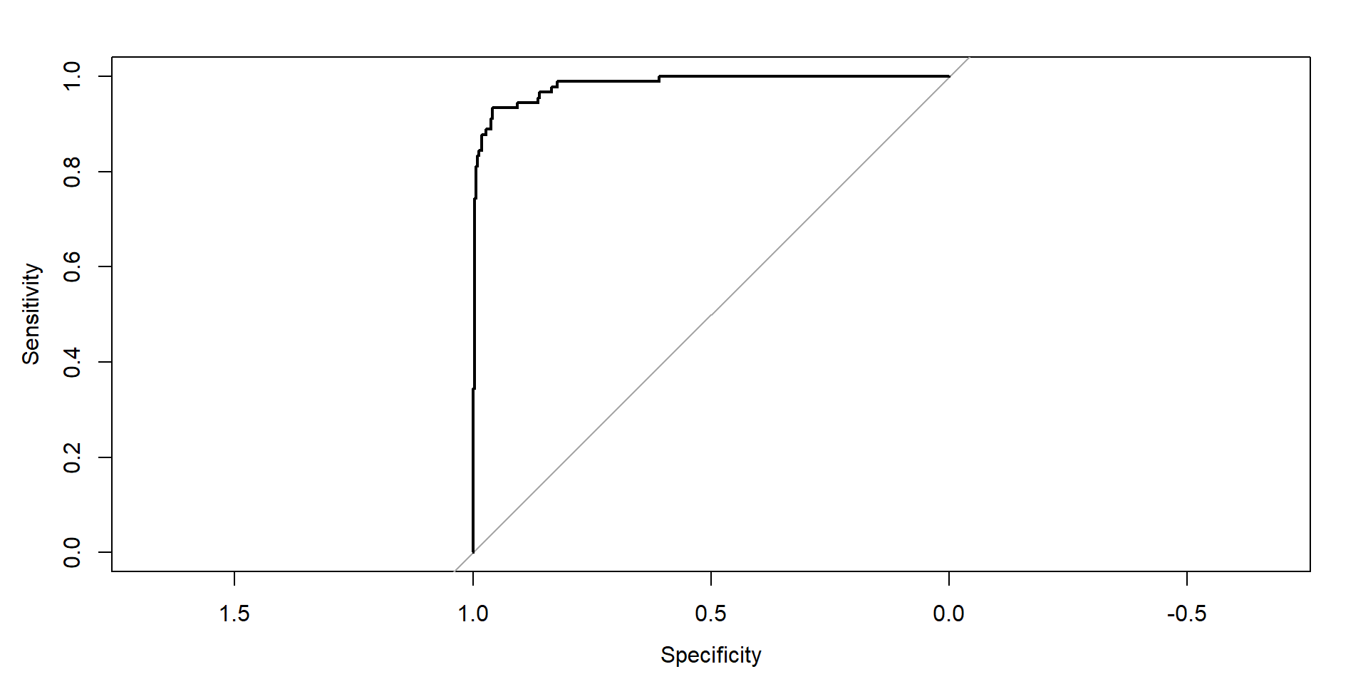
rocc_glmnet <- pROC::roc(data_eval_ttt_2, response="truth", predictor="prob.suspect_glmnet", levels=c("normal", "suspect"))

rocc_ranger <- pROC::roc(data_eval_ttt_2, response="truth", predictor="prob.suspect_ranger", levels=c("normal", "suspect"))

plot(rocc_glmnet, col="blue")
plot(rocc_ranger, add=TRUE, col="orange")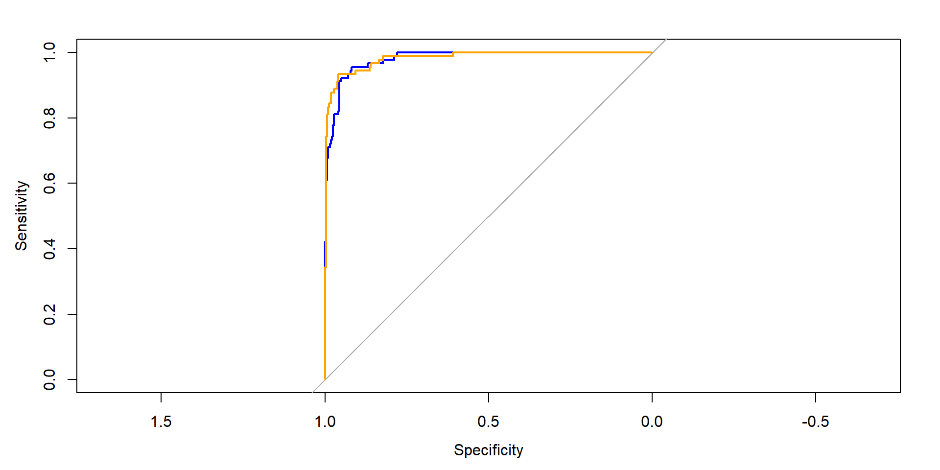

CI for difference in AUCs (Delong)

pROC::roc.test(rocc_ranger, rocc_glmnet, 
               paired=TRUE, method="delong")


    DeLong's test for two correlated ROC curves

data:  rocc_ranger and rocc_glmnet
Z = 0.40273, p-value = 0.6871
alternative hypothesis: true difference in AUC is not equal to 0
95 percent confidence interval:
 -0.009339915  0.014170832
sample estimates:
AUC of roc1 AUC of roc2 
  0.9830918   0.9806763

CI for difference in AUCs (bootstrap)

pROC::roc.test(rocc_ranger, rocc_glmnet, 
               paired=TRUE, method="bootstrap")


    Bootstrap test for two correlated ROC curves

data:  rocc_ranger and rocc_glmnet
D = 0.39739, boot.n = 2000, boot.stratified = 1, p-value = 0.6911
alternative hypothesis: true difference in AUC is not equal to 0
sample estimates:
AUC of roc1 AUC of roc2 
  0.9830918   0.9806763

UQ for (nested) CV

Scenario: Algorithm evaluation or comparison in the outer loop of nested CV
- glmnet, ranger were tuned in the inner loop
- comparison of best hyperparameter combination of each approach
- on each fold (1:5), compare model that was trained on remaining observations

How can we quantify uncertainty for (difference of) performance estimate?

A few recommendations do exist (Raschka, 2018)
We will focus again on the bootstrap and a hierarchical bootstrap variant

UQ for (nested) CV

head(data_eval_ncv_2)

   fold row_ids  truth response_glmnet prob.suspect_glmnet prob.normal_glmnet
1:    1       3 normal          normal        3.057173e-02          0.9694283
2:    1      15 normal          normal        4.057469e-04          0.9995943
3:    1      27 normal          normal        7.387341e-07          0.9999993
4:    1      30 normal          normal        1.959313e-04          0.9998041
5:    1      33 normal          normal        1.123090e-04          0.9998877
6:    1      34 normal          normal        8.422928e-04          0.9991577
   response_ranger prob.suspect_ranger prob.normal_ranger
1:          normal         0.306187443          0.6938126
2:          normal         0.000000000          1.0000000
3:          normal         0.001503821          0.9984962
4:          normal         0.004442368          0.9955576
5:          normal         0.004255131          0.9957449
6:          normal         0.000000000          1.0000000

UQ for (nested) CV - bootstrap approaches

Simple bootstrap
- resample observations/rows of original evaluation data with replacement
- apply function (metric/statistic) to each resampled dataset
- repeat…

Hierarchical bootstrap
- resample fold id (in this case 1:5) with replacement
- resample observations within these folds with replacement
- apply function (metric/statistic) to each resampled dataset
- repeat…

UQ for (nested) CV - hierarchical bootstrap in R

fabricatr::resample_data(data_eval_ncv_2,
                         N=c(n_fold, n_obs_per_fold),
                         ID_labels = c("fold", "row_ids"))

UQ for (nested) CV - bootstrap approaches

summary(resampled_cv_simple$delta)

   Min. 1st Qu.  Median    Mean 3rd Qu.    Max. 
0.01122 0.02110 0.02334 0.02344 0.02568 0.03747

summary(resampled_cv_nested$delta)

    Min.  1st Qu.   Median     Mean  3rd Qu.     Max. 
0.008422 0.020422 0.023595 0.023605 0.026817 0.040722

UQ for (nested) CV - bootstrap approaches

delta = AUC(ranger) - AUC(glmnet)
quantile computation below amounts to type “percentile” in boot::boot.ci

quantile(resampled_cv_simple$delta, c(0.025, 0.975))

      2.5%      97.5% 
0.01693917 0.03068130

quantile(resampled_cv_nested$delta, c(0.025, 0.975))

      2.5%      97.5% 
0.01454324 0.03271745

Multiple metrics

Usually no multiplicity correction when multiple metrics are assesed (one per performance dimension: discrimination, calibration, …)
per performance dimension:
- define primary metric of interest
- additional secondary metrics can be investigated

Train-tune-test with single “test” model

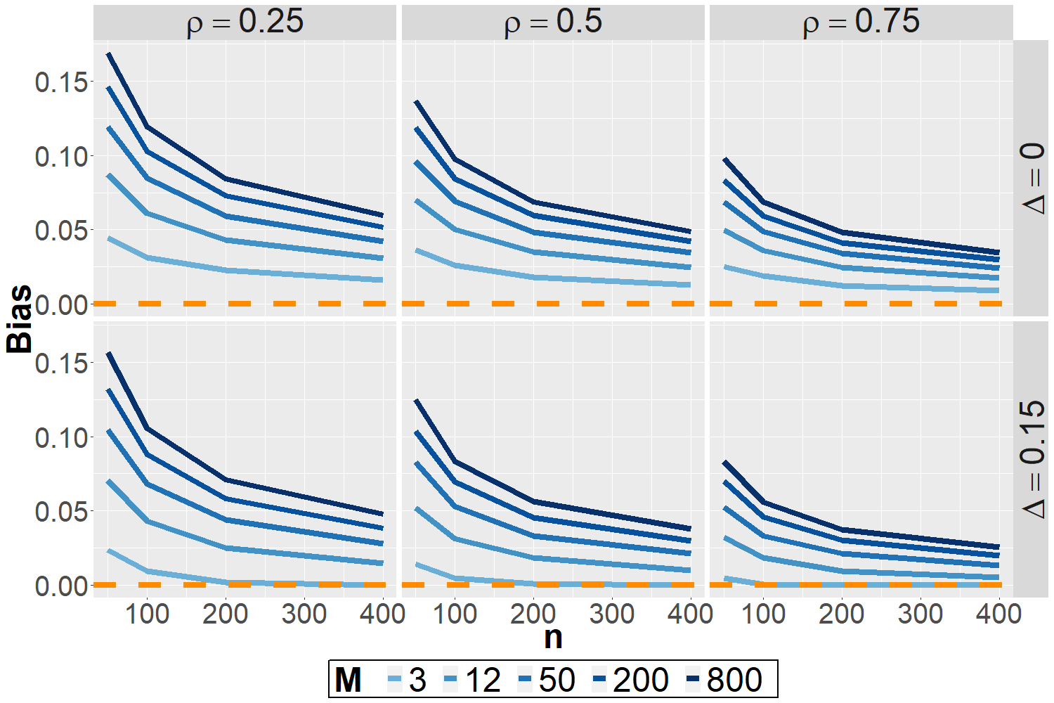
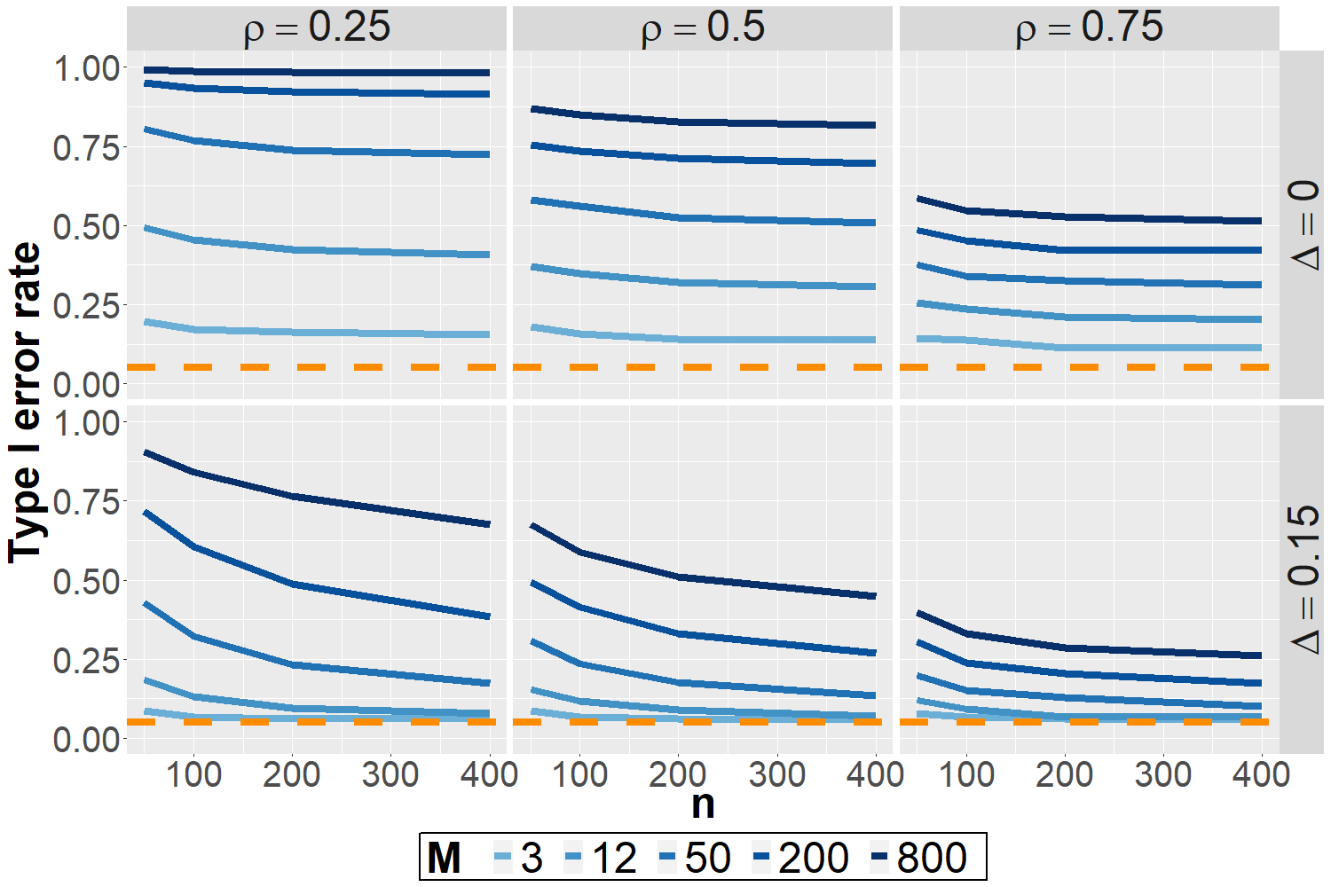
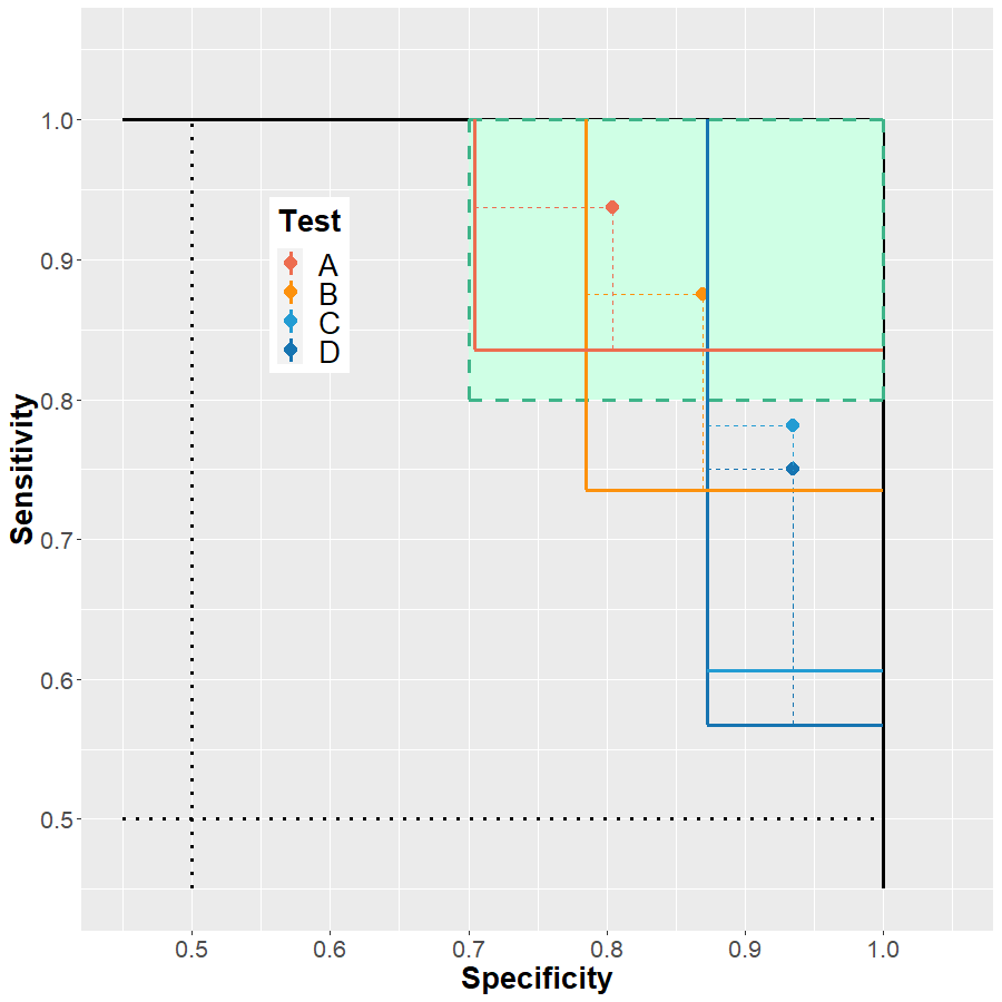
Train-tune-test with multiple comparisons

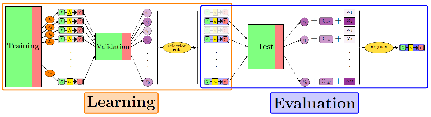
Multiple models, multiple metrics

Interactive summary

Q1: What is NOT a typical goal of the statistical analysis in ML evaluation studies?

hyperparameter optimization
performance estimation
hypothesis testing
uncertainty quantification

Q1: What is NOT a typical goal of the statistical analysis in ML evaluation studies?

hyperparameter optimization
performance estimation
hypothesis testing
uncertainty quantification

Q2: Which is a valid choice of a comparator?

another performance metric
another prediction model
a fixed threshold
none

Q2: Which is a valid choice of a comparator?

another performance metric
another prediction model
a fixed threshold
none

Q3: The classical boostrap should in general NOT be used…

for resampling / data splitting
as part of learning algorithms
for uncertainty quantification in simple scenarios
for statistical anaylsis of hierarchical data

Q3: The classical boostrap should in general NOT be used…

for resampling / data splitting
as part of learning algorithms
for uncertainty quantification in simple scenarios
for statistical anaylsis of hierarchical data

Q4: Multiple models should not be assessed on the test dataset, unless…

they are all trained by the same learning algorithm
they have been developed by different persons/groups
a correction for multiple comparisons is employed
the paper will be submitted to “Nature Machine Intelligence”

Q4: Multiple models should not be assessed on the test dataset, unless…

they are all trained by the same learning algorithm
they have been developed by different persons/groups
a correction for multiple comparisons is employed
the paper will be submitted to “Nature Machine Intelligence”

Questions

Practical aspects

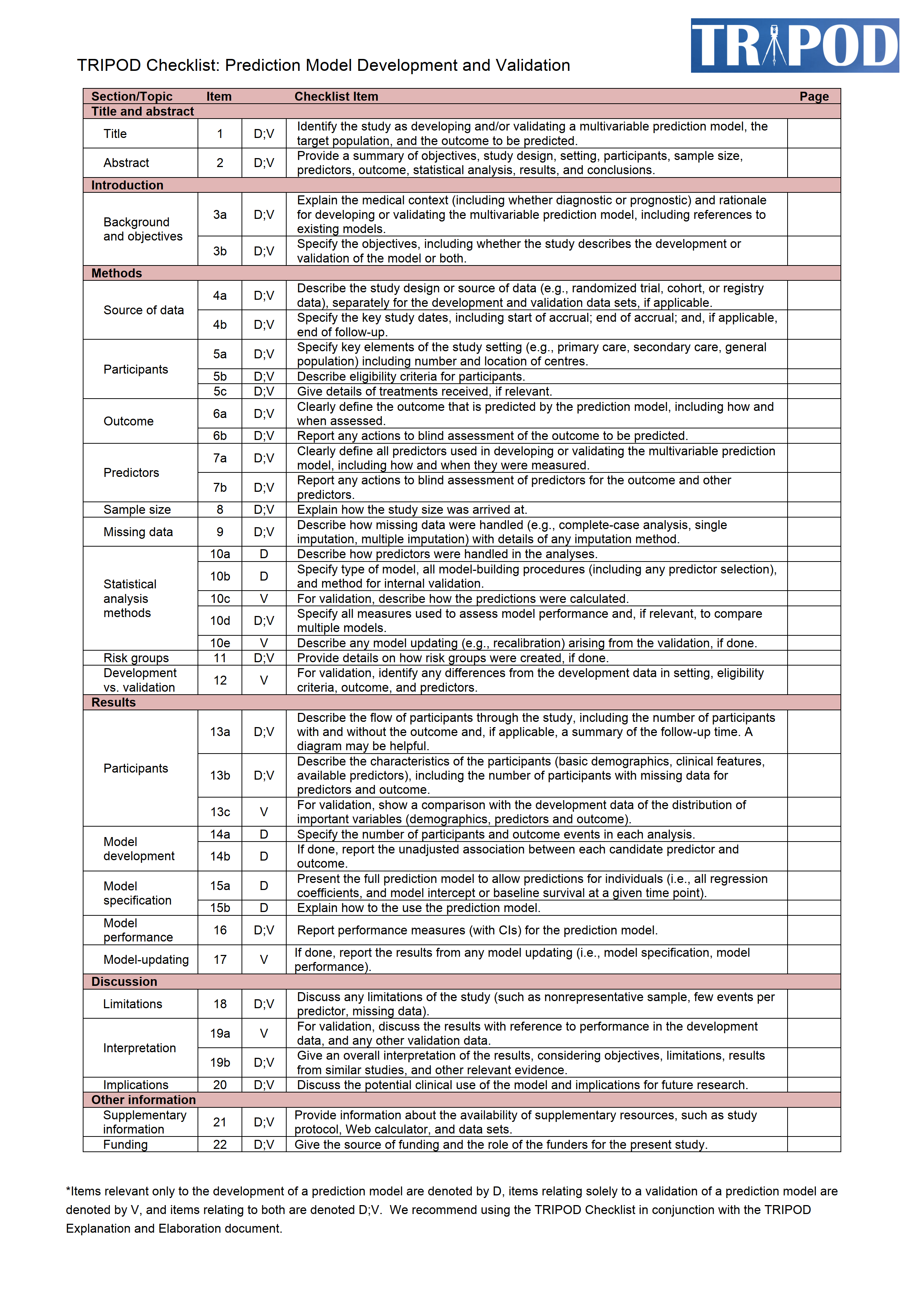
Reporting guidelines

TRIPOD: Transparent reporting of a multivariable prediction model for individual prognosis or diagnosis (TRIPOD): The TRIPOD statement (2015)
TRIPOD-AI (in preparation)
REFORMS: Reporting Standards for ML-based Science (2023)

TRIPOD

Planning ahead

flowchart LR
  MS(Metric selection) --> SA(Statistical analysis)
  DS(Data splitting) --> SA
  SA --> R(Reporting)

Study protocol (e.g. for prospective data aquisition)
Statistical analysis plan

Project organization

The “conflict of interest” of applied ML
- we want high numbers (empirical performance estimates)
- we want meaningful numbers (e.g. unbiased estimates)

Splitting up work for development, evaluation (between persons, teams, institutions) makes things a whole lot easier
- different teams should still work together
- a good evaluation effort can support model development

Requirement analysis

Typical requirements for ML solutions
- need for predicted probabilities
- sufficient interpretability (limited complexity)
- fast inference speed
- …

Requirements should be assessed initially, not after performance evaluation.
This usually requires discussion with domain experts.

Power calculation

Power: probability to be able to demonstrate suitability of a/your (new) model/algorithm
For evaluation on test set after training and tuning: a wide variety of methods exists (classification \(\leftrightarrow\) diagnostic accuracy studies)
- Hypothesis testing based
- Precision based, e.g. here: https://shiny.ctu.unibe.ch/app_direct/presize/

Target population/setting

What is the target population/setting?
- Define sensible inclusion/exclusion criteria
- Helps to assemble the test set (IEC are met)

During development, things may well be (and often are) a little “wilder”:
- Synthetic data
- Transfer learning (other population/setting)
- Data augmentation (e.g. manipulation of medical images)

None of these is sensible in an evaluation context!
Exception: sensitivity analyses…

Reproducibility

Reproducibility is important but also hard (in particular in ML)
- many sources of variability
- volatile software packages
- non-deterministic learning

Some practical considerations
- random seed(ing) (set.seed(123))
- version control (e.g. github)
- experiment handling (e.g. batchtools package)
- pipeline management (e.g. targets package)

Interactive summary

Q1: What is NOT a reporting guideline for predictive modelling studies?

TRIPOD
TRIPOD-AI
REPORT-AI
REFORMS

Q1: What is NOT a reporting guideline for predictive modelling studies?

TRIPOD
TRIPOD-AI
REPORT-AI
REFORMS

Q2: What is mostly NOT depending on the other options and should thus be decided upon initially?

data splitting
statistical analysis
metric selection
reporting

Q2: What is mostly NOT depending on the other options and should thus be decided upon initially?

data splitting
statistical analysis
metric selection
reporting

Q3: The “conflict of interest of predictive modelling” can be (partially) avoided by…

avoiding any claims on statistical significance
separating model development and model evaluation
adequate & transparent study planning
intransparent reporting

Q3: The “conflict of interest of predictive modelling” can be (partially) avoided by…

avoiding any claims on statistical significance
separating model development and model evaluation
adequate & transparent study planning
intransparent reporting

Q4: Power analyses…

can help to avoid conducting unreasonably large studies
are independent of the chosen evaluation metric
are only useful if hypothesis testing is planned for evaluation
should be reported according to the TRIPOD statement

Q4: Power analyses…

can help to avoid conducting unreasonably large studies
are independent of the chosen evaluation metric
are only useful if hypothesis testing is planned for evaluation
should be reported according to the TRIPOD statement

Q5: For prospective studies, additional care is required…

to avoid leakage
to avoid statistically significant results
to end up with an adequate test set
to define the performance metric(s)

Q5: For prospective studies, additional care is required…

to avoid leakage
to avoid statistically significant results
to end up with an adequate test set
to define the performance metric(s)

Questions

Wrap-up

Learnings

Several pitfalls are very prevalent in applied ML.
Overfitting and selection-induced bias cause overoptimistic evaluation results.
Performance metric(s) should be chosen deliberately.
Multiple dimensions can/should to be considered: discrimination, calibration, fairness, …
Calibration is usually harder to achieve than discrimination.
Data splitting is mandatory to avoid overoptimism.
Large(r) samples: train-tune-test \(\rightarrow\) simple(r).
Fewe(r) samples: (nested) CV (+test) \(\rightarrow\) (more) complex.
Statistical analysis depends on metric choice and data splitting approach.
Bootstrap can deal with any metric and requires minimal assumptions.
Plan ahead (requirement analysis) and involve important stakeholders.
Evaluation should guide/support development.

Contact

- Feedback
- Further questions
- Collaboration requests
@MaxWestphal89
- Get/stay in touch
https://github.com/maxwestphal/evaluation_in_supervised_ml_cen_2023/issues
- Issues with slides/code

Have 10 minutes to spare?

In a current research project, we develop an interactive expert system for methodological guidance in applied ML (beyond model evaluation).
We have setup a short survey to assess user needs and requirements.
Thank you for your time!

https://websites.fraunhofer.de/mlguide-user-survey/index.php/578345/newtest/Y?G00Q23=CEN23

Thank you for your participation! Have a great conference!