2  Results

Code

library(dplyr)

Attaching package: 'dplyr'

The following objects are masked from 'package:stats':

    filter, lag

The following objects are masked from 'package:base':

    intersect, setdiff, setequal, union

Code

library(ggplot2)

Code

knitr::opts_chunk$set(cache=FALSE)

Code

owntheme <- theme(legend.position = "bottom",
                  title=element_text(face="bold", size=24),
                  axis.title = element_text(face="bold", size=20),
                  legend.text = element_text(face="plain", size=20),
                  legend.title = element_blank(), 
                  axis.text = element_text(size=16)) 

Code

## set input dir, needs to be equal to out.dir from
## cases_simstudy_lfc.R and cases_simstudy_roc.R:
in.dir <- file.path("E:/cases_simstudy/cases_sim_results")

For local reproduction, the input directory potentially needs to be adapted!

2.1 Simulation study 1: LFC setting

2.1.1 Main results

Code

data_lfc <- readr::read_csv2(file.path(in.dir, "cases_SIM_LFC.csv"))

ℹ Using "','" as decimal and "'.'" as grouping mark. Use `read_delim()` for more control.

Rows: 5600000 Columns: 61
── Column specification ────────────────────────────────────────────────────────
Delimiter: ";"
chr (10): problem, algorithm, cortype, contrast, alternative, adjustment, tr...
dbl (50): job.id, nrep, n, prev, m, se, sp, L, rhose, rhosp, benchmark, alph...
lgl  (1): random

ℹ Use `spec()` to retrieve the full column specification for this data.
ℹ Specify the column types or set `show_col_types = FALSE` to quiet this message.

Code

data_lfc <- data_lfc %>%
  mutate(Adjustment = recode_factor(
    interaction(adjustment, pars),
    "none.list()" = "none",
    "bonferroni.list()"="Bonferroni", 
    "maxt.list()" = "maxT",
    "mbeta.list()" = "mBeta",
    "bootstrap.list(type='wild')" = "Bootstrap (wild)",
    "bootstrap.list()" = "Bootstrap (pairs)")
  )

dim(data_lfc)

[1] 5600000      62

Code

data_lfc <- data_lfc %>% 
  filter(cortype == "equi") %>% 
  filter(rhose == 0.5) %>%
  filter(transformation == "none") 

dim(data_lfc)

[1] 2400000      62

Code

data_lfc %>% 
  filter(n<1000, prev==0.25, se==0.8, m==10) %>%
  group_by(Adjustment, n, prev, se, m) %>%
  summarize(nsim=n(), rr = mean(`0` > 0)) %>%
  ggplot(aes(n, rr, col=Adjustment, fill=Adjustment, pch=Adjustment))+
  geom_point(size=6, alpha=0.6) +
  geom_line(size=2, alpha=0.6) +
  xlab("Total sample size") +
  ylab("FWER") +
  scale_shape_manual(values = c(21, 22, 24, 25, 23, 23)) +
  geom_hline(yintercept=0.025, col="red", lwd=2, lty=2, alpha=0.75) +
  owntheme

`summarise()` has grouped output by 'Adjustment', 'n', 'prev', 'se'. You can
override using the `.groups` argument.

Warning: Using `size` aesthetic for lines was deprecated in ggplot2 3.4.0.
ℹ Please use `linewidth` instead.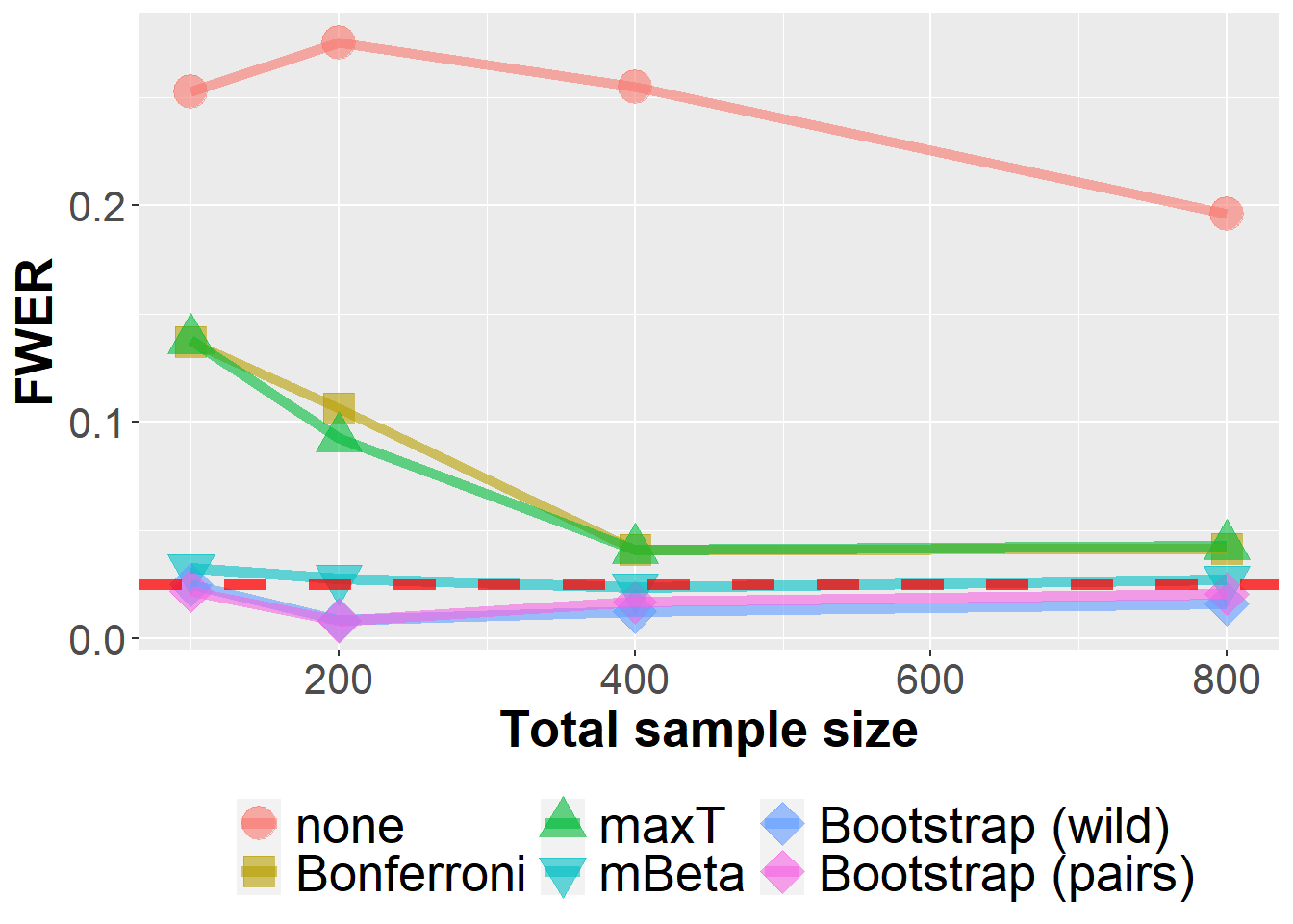

Code

data_lfc %>% 
  filter(n<1000, prev==0.25, se==0.8, m==10) %>%
  group_by(Adjustment, n, prev, se, m) %>%
  summarize(nsim=n(), rr = mean(`0.05` > 0)) %>%
  ggplot(aes(n, rr, col=Adjustment, fill=Adjustment, pch=Adjustment)) +
  geom_point(size=6, alpha=0.6) +
  geom_line(size=2, alpha=0.6) +
  xlab("Total sample size") +
  ylab("Power") + 
  scale_shape_manual(values = c(21, 22, 24, 25, 23, 23)) +
  owntheme

`summarise()` has grouped output by 'Adjustment', 'n', 'prev', 'se'. You can
override using the `.groups` argument.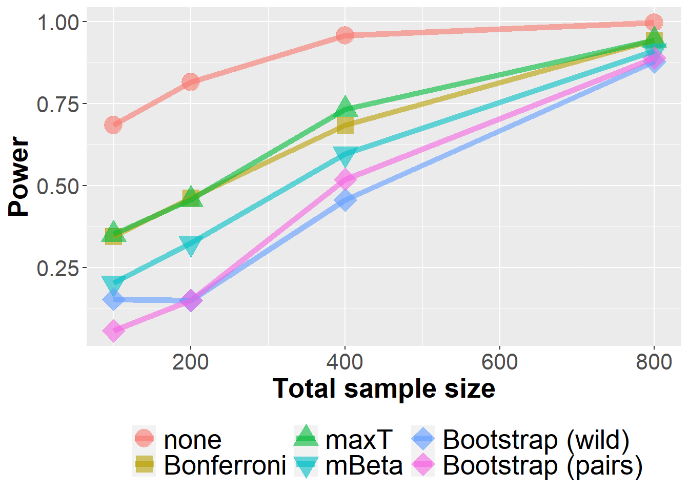

2.1.2 Sensitivity analyses

Code

data_lfc %>% 
  filter(n<1000) %>%
  group_by(Adjustment, n, prev, se, m) %>%
  summarize(nsim=n(), rr = mean(`0` > 0)) %>%
  ggplot(aes(n, rr, col=Adjustment, fill=Adjustment, pch=Adjustment))+
  geom_point(size=6, alpha=0.6) +
  geom_line(size=2, alpha=0.6) +
  xlab("Total sample size") +
  ylab("FWER") +
  scale_shape_manual(values = c(21, 22, 24, 25, 23, 23)) +
  geom_hline(yintercept=0.025, col="red", lwd=2, lty=2, alpha=0.75) +
  owntheme +
  facet_wrap(prev+se ~ m, ncol=2, 
             labeller = label_bquote("prev = " ~ .(prev) * ", " * "se = " ~ .(se) * ", " * "m = " ~ .(m)))

`summarise()` has grouped output by 'Adjustment', 'n', 'prev', 'se'. You can
override using the `.groups` argument.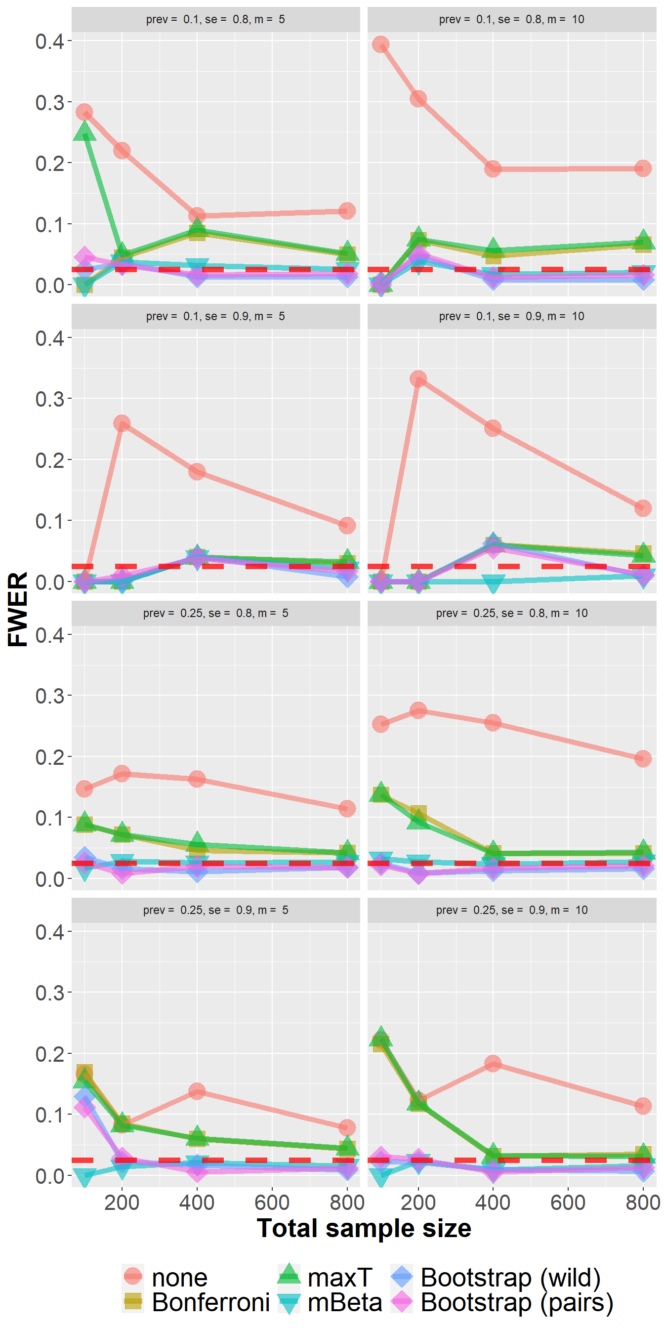

Code

data_lfc %>% 
  filter(n<1000) %>%
  group_by(Adjustment, n, prev, se, m) %>%
  summarize(nsim=n(), rr = mean(`0.05` > 0)) %>%
  ggplot(aes(n, rr, col=Adjustment, fill=Adjustment, pch=Adjustment)) +
  geom_point(size=6, alpha=0.6) +
  geom_line(size=2, alpha=0.6) +
  xlab("Total sample size") +
  ylab("Power") + 
  scale_shape_manual(values = c(21, 22, 24, 25, 23, 23)) +
  owntheme +
  facet_wrap(prev+se ~ m, ncol=2, 
             labeller = label_bquote("prev = " ~ .(prev) * ", " * "se = " ~ .(se) * ", " * "m = " ~ .(m)))

`summarise()` has grouped output by 'Adjustment', 'n', 'prev', 'se'. You can
override using the `.groups` argument.

Code

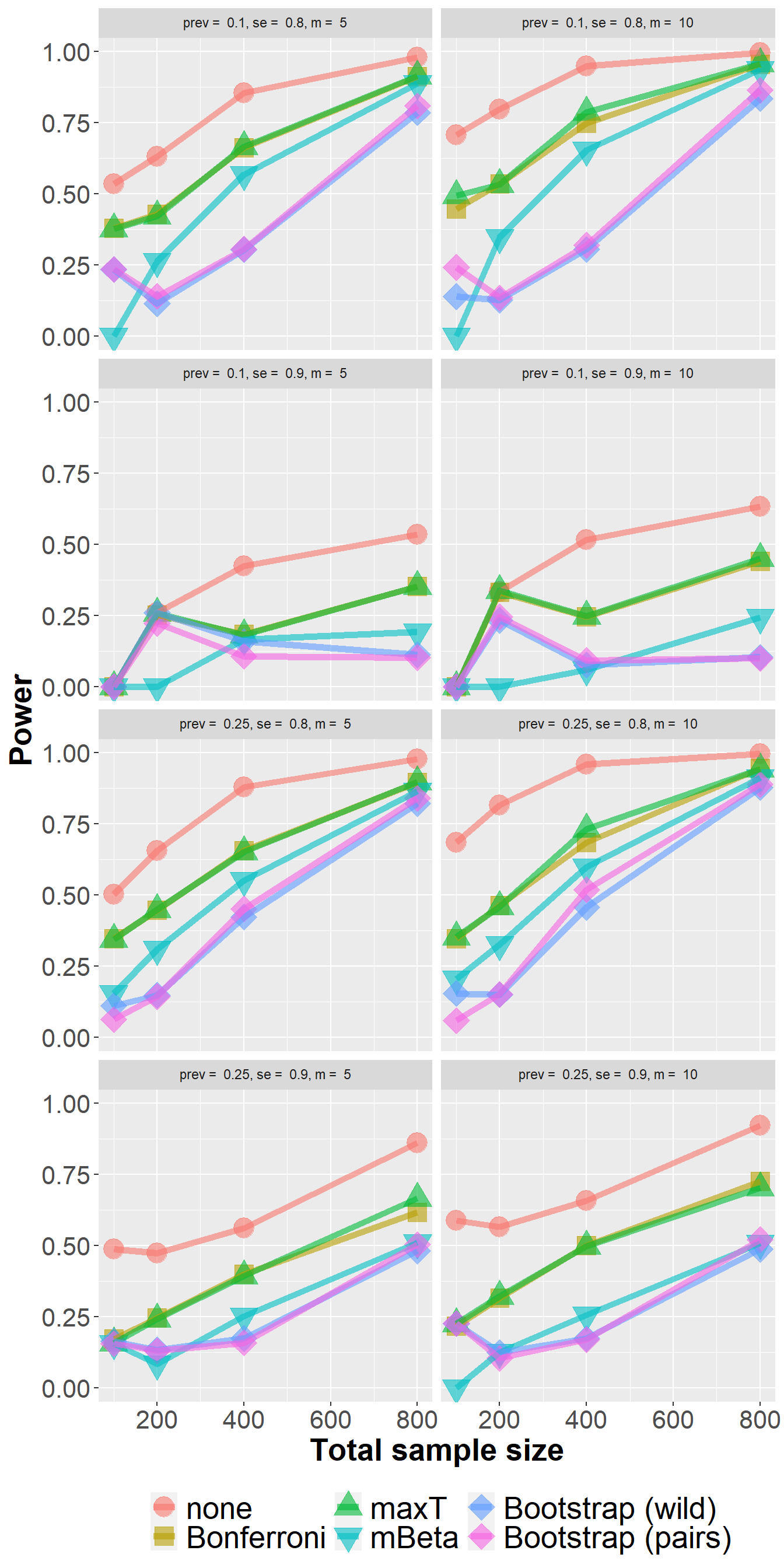
data_lfc %>% 
  filter(n<1000) %>%
  group_by(Adjustment, n, prev, se, m) %>%
  summarize(nsim=n(), rr = mean(`0.1` > 0)) %>%
  ggplot(aes(n, rr, col=Adjustment, fill=Adjustment, pch=Adjustment)) +
  geom_point(size=6, alpha=0.6) +
  geom_line(size=2, alpha=0.6) +
  xlab("Total sample size") +
  ylab("Power") + 
  scale_shape_manual(values = c(21, 22, 24, 25, 23, 23)) +
  owntheme +
  facet_wrap(prev+se ~ m, ncol=2, 
             labeller = label_bquote("prev = " ~ .(prev) * ", " * "se = " ~ .(se) * ", " * "m = " ~ .(m)))

`summarise()` has grouped output by 'Adjustment', 'n', 'prev', 'se'. You can
override using the `.groups` argument.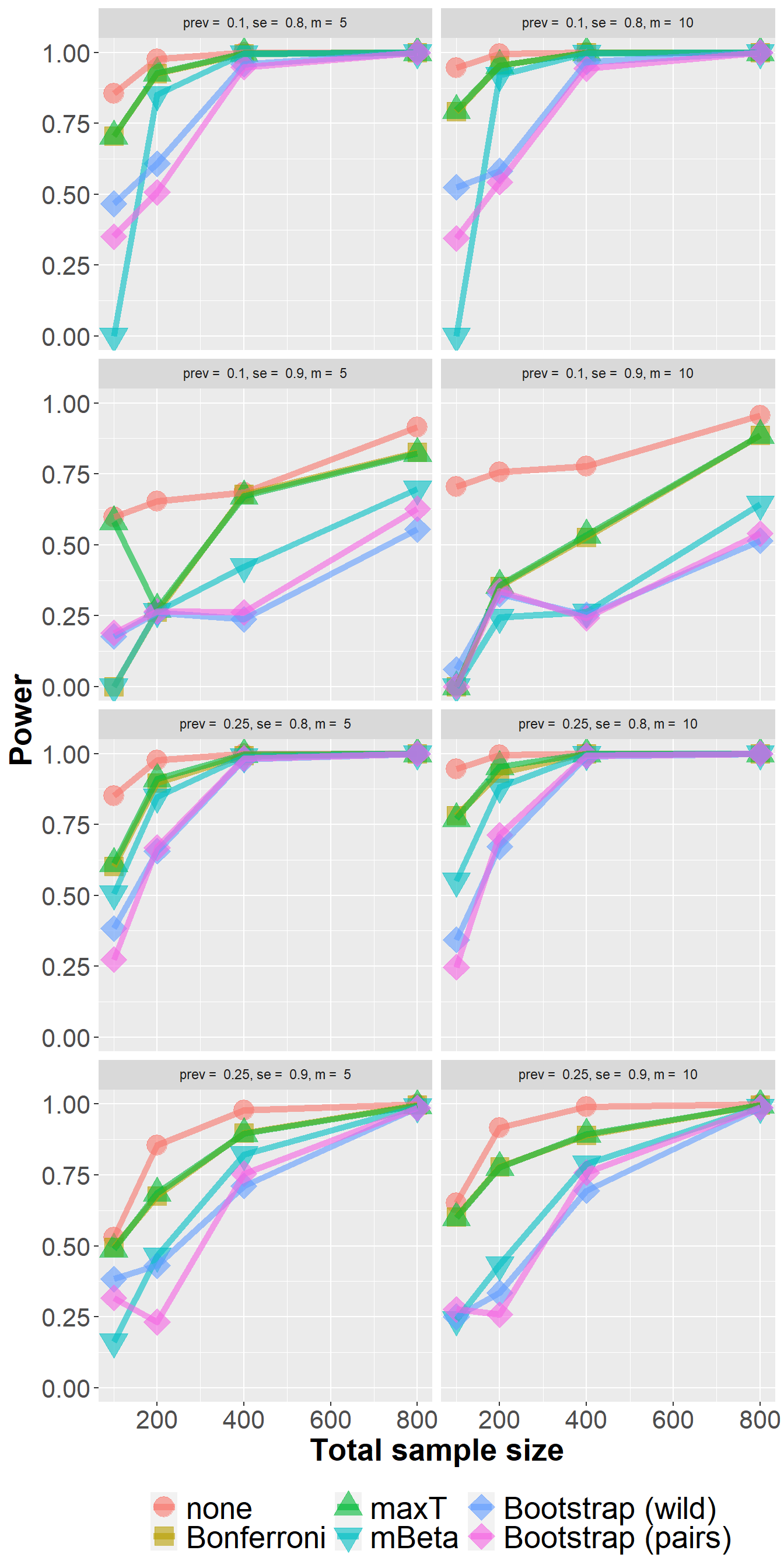

2.2 Simulation study 2: ROC setting

2.2.1 Main results

Code

data_roc <- readr::read_csv2(file.path(in.dir, "cases_SIM_ROC.csv"))

ℹ Using "','" as decimal and "'.'" as grouping mark. Use `read_delim()` for more control.

Rows: 8400000 Columns: 61
── Column specification ────────────────────────────────────────────────────────
Delimiter: ";"
chr (10): problem, algorithm, auc, contrast, alternative, adjustment, transf...
dbl (50): job.id, nrep, n, prev, m, rhose, e, k, delta, rhosp, benchmark, al...
lgl  (1): random

ℹ Use `spec()` to retrieve the full column specification for this data.
ℹ Specify the column types or set `show_col_types = FALSE` to quiet this message.

Code

data_roc <- data_roc %>%
  mutate(Adjustment = recode_factor(
    interaction(adjustment, pars),
    "none.list()" = "none",
    "bonferroni.list()"="Bonferroni", 
    "maxt.list()" = "maxT",
    "mbeta.list()" = "mBeta",
    "bootstrap.list(type='wild')" = "Bootstrap (wild)",
    "bootstrap.list()" = "Bootstrap (pairs)")
  )

dim(data_roc)

[1] 8400000      62

Code

data_roc <- data_roc %>% 
  filter(rhose == 0.5) %>%
  filter(auc == "seq(0.85, 0.90, length.out = 5)") %>% 
  filter(transformation == "none") 

dim(data_roc)

[1] 1200000      62

Code

data_roc %>% 
  filter(n<1000, prev==0.25, m==10) %>%
  group_by(Adjustment, n, prev, m) %>%
  summarize(nsim=n(), rr = mean(`0` > 0)) %>%
  ggplot(aes(n, rr, col=Adjustment, fill=Adjustment, pch=Adjustment))+
  geom_point(size=6, alpha=0.6) +
  geom_line(size=2, alpha=0.6) +
  xlab("Total sample size") +
  ylab("FWER") +
  scale_shape_manual(values = c(21, 22, 24, 25, 23, 23)) +
  geom_hline(yintercept=0.025, col="red", lwd=2, lty=2, alpha=0.75) +
  owntheme 

`summarise()` has grouped output by 'Adjustment', 'n', 'prev'. You can override
using the `.groups` argument.

Code

data_roc %>% 
  filter(n<1000, prev==0.25, m==10) %>%
  group_by(Adjustment, n, prev, m) %>%
  summarize(nsim=n(), rr = mean(`0.1` > 0)) %>%
  ggplot(aes(n, rr, col=Adjustment, fill=Adjustment, pch=Adjustment)) +
  geom_point(size=6, alpha=0.6) +
  geom_line(size=2, alpha=0.6) +
  xlab("Total sample size") +
  ylab("Power") + 
  scale_shape_manual(values = c(21, 22, 24, 25, 23, 23)) +
  owntheme 

`summarise()` has grouped output by 'Adjustment', 'n', 'prev'. You can override
using the `.groups` argument.

2.2.2 Sensitivity analyses

Code

data_roc %>% 
  filter(n<1000) %>%
  group_by(Adjustment, n, prev, m) %>%
  summarize(nsim=n(), rr = mean(`0` > 0)) %>%
  ggplot(aes(n, rr, col=Adjustment, fill=Adjustment, pch=Adjustment))+
  geom_point(size=6, alpha=0.6) +
  geom_line(size=2, alpha=0.6) +
  xlab("Total sample size") +
  ylab("FWER") +
  scale_shape_manual(values = c(21, 22, 24, 25, 23, 23)) +
  geom_hline(yintercept=0.025, col="red", lwd=2, lty=2, alpha=0.75) +
  owntheme +
  facet_wrap(prev ~ m, ncol=2, 
             labeller = label_bquote("prev = " ~ .(prev) * ", " * "m = " ~ .(m)))

`summarise()` has grouped output by 'Adjustment', 'n', 'prev'. You can override
using the `.groups` argument.

Code

data_roc %>% 
  filter(n<1000) %>%
  group_by(Adjustment, n, prev, m) %>%
  summarize(nsim=n(), rr = mean(`0.1` > 0)) %>%
  ggplot(aes(n, rr, col=Adjustment, fill=Adjustment, pch=Adjustment)) +
  geom_point(size=6, alpha=0.6) +
  geom_line(size=2, alpha=0.6) +
  xlab("Total sample size") +
  ylab("Power") + 
  scale_shape_manual(values = c(21, 22, 24, 25, 23, 23)) +
  owntheme +
  facet_wrap(prev ~ m, ncol=2, 
             labeller = label_bquote("prev = " ~ .(prev) * ", " * "m = " ~ .(m)))

`summarise()` has grouped output by 'Adjustment', 'n', 'prev'. You can override
using the `.groups` argument.

Code

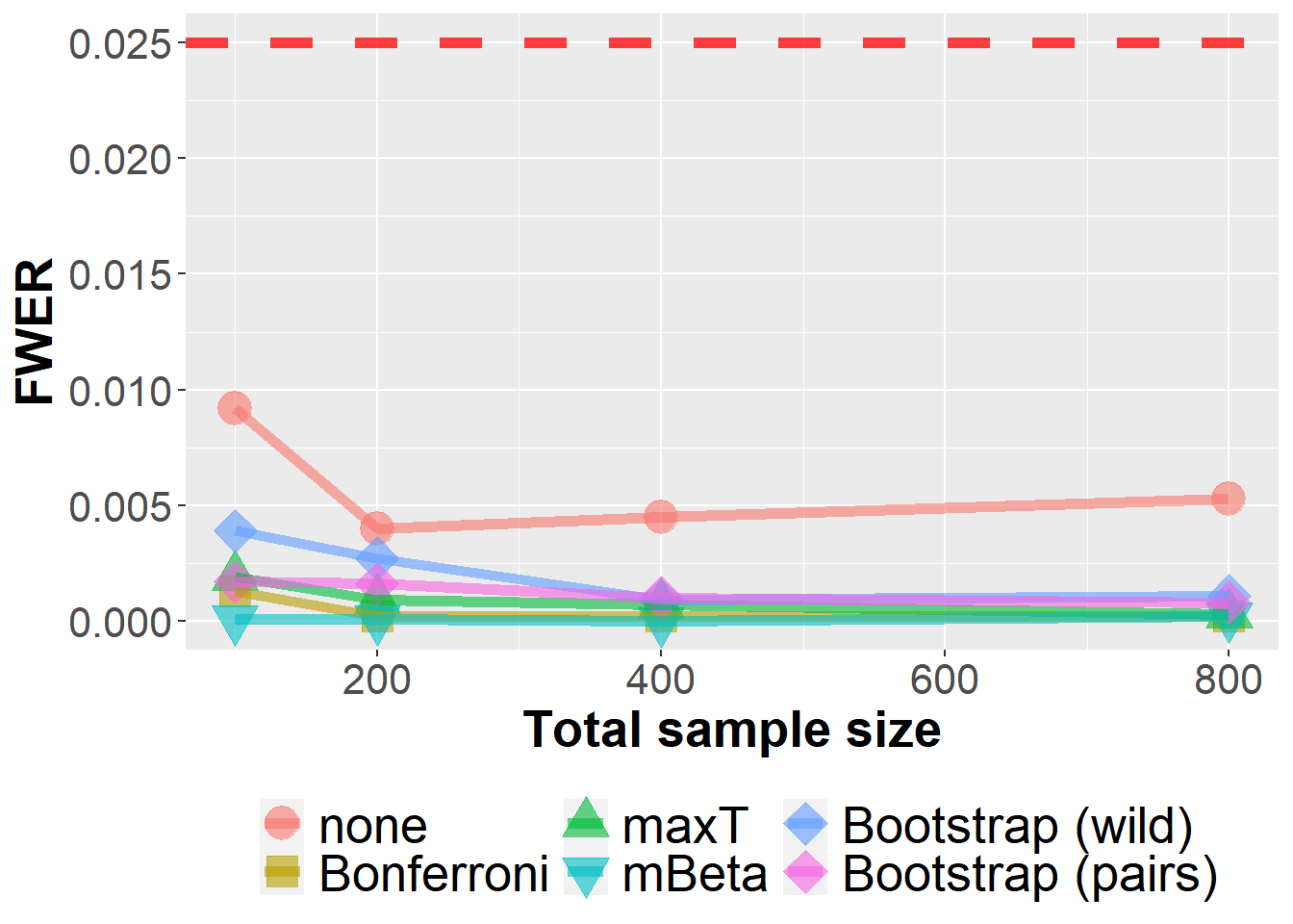
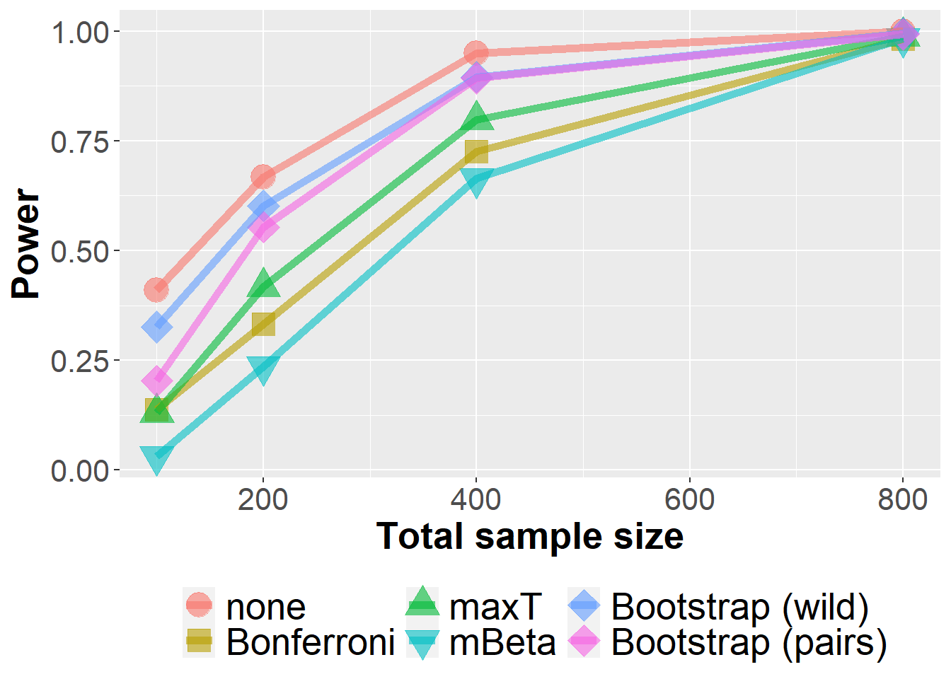
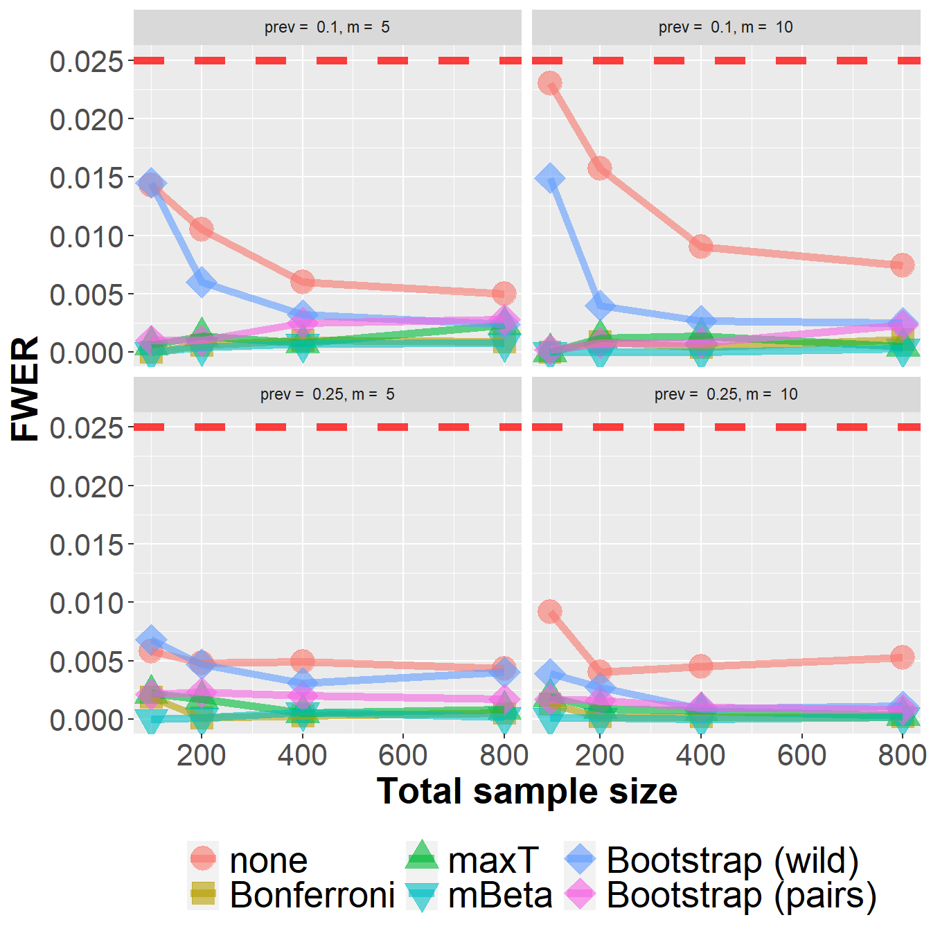
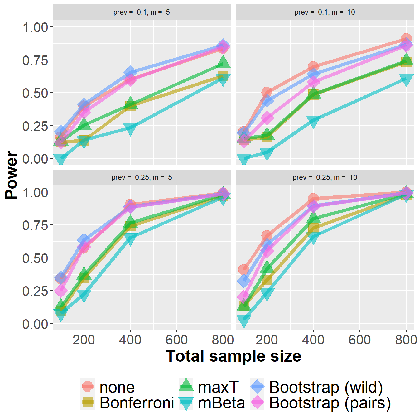
data_roc %>% 
  filter(n<1000) %>%
  group_by(Adjustment, n, prev, m) %>%
  summarize(nsim=n(), rr = mean(`0.05` > 0)) %>%
  ggplot(aes(n, rr, col=Adjustment, fill=Adjustment, pch=Adjustment)) +
  geom_point(size=6, alpha=0.6) +
  geom_line(size=2, alpha=0.6) +
  xlab("Total sample size") +
  ylab("Power") + 
  scale_shape_manual(values = c(21, 22, 24, 25, 23, 23)) +
  owntheme +
  facet_wrap(prev ~ m, ncol=2, 
             labeller = label_bquote("prev = " ~ .(prev) * ", " * "m = " ~ .(m)))

`summarise()` has grouped output by 'Adjustment', 'n', 'prev'. You can override
using the `.groups` argument.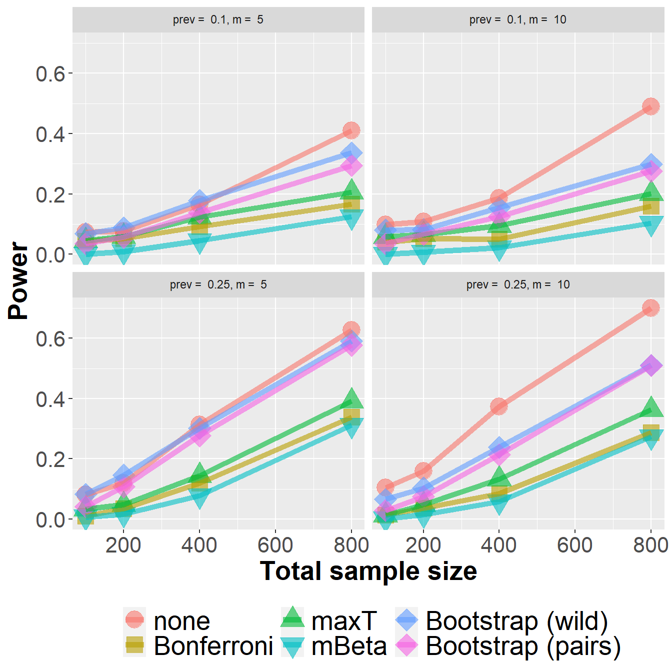

2.3 Simulation study 3: Further sensitivity analyses

Code

in.dir <- file.path("E:/cases_SIM/cases_SIM_results") # TODO: remove

data_sens_lfc <- readr::read_csv2(file.path(in.dir, "cases_SIM_SENS_lfc.csv"))

ℹ Using "','" as decimal and "'.'" as grouping mark. Use `read_delim()` for more control.

Rows: 400000 Columns: 61
── Column specification ────────────────────────────────────────────────────────
Delimiter: ";"
chr (10): problem, algorithm, cortype, contrast, alternative, adjustment, tr...
dbl (50): job.id, nrep, n, prev, m, se, sp, L, rhose, rhosp, benchmark, alph...
lgl  (1): random

ℹ Use `spec()` to retrieve the full column specification for this data.
ℹ Specify the column types or set `show_col_types = FALSE` to quiet this message.

Code

data_sens_lfc <- data_sens_lfc %>%
  mutate(Adjustment = recode_factor(
    interaction(adjustment, pars, drop = TRUE),
    "none.list()" = "none",
    "bonferroni.list()"="Bonferroni", 
    "maxt.list()" = "maxT",
    "mbeta.list()" = "mBeta (lfc_pr=1)",
    "mbeta.list(lfc_pr=0.5)" = "mBeta (lfc_pr=0.5)",
    "mbeta.list(lfc_pr=0)" = "mBeta (lfc_pr=0)",
    "bootstrap.list(type='wild')" = "Bootstrap (wild)",
    "bootstrap.list()" = "Bootstrap (pairs)") 
  )

dim(data_sens_lfc)

[1] 400000     62

Code

data_sens_roc <- readr::read_csv2(file.path(in.dir, "cases_SIM_SENS_roc.csv"))

ℹ Using "','" as decimal and "'.'" as grouping mark. Use `read_delim()` for more control.

Rows: 800000 Columns: 62
── Column specification ────────────────────────────────────────────────────────
Delimiter: ";"
chr (11): problem, algorithm, auc, dist, contrast, alternative, adjustment, ...
dbl (50): job.id, nrep, n, prev, m, rhose, e, k, delta, rhosp, benchmark, al...
lgl  (1): random

ℹ Use `spec()` to retrieve the full column specification for this data.
ℹ Specify the column types or set `show_col_types = FALSE` to quiet this message.

Code

data_sens_roc <- data_sens_roc %>%
  mutate(Adjustment = recode_factor(
    interaction(adjustment, pars, drop = TRUE),
    "none.list()" = "none",
    "bonferroni.list()"="Bonferroni", 
    "maxt.list()" = "maxT",
    "mbeta.list()" = "mBeta (lfc_pr=1)",
    "mbeta.list(lfc_pr=0.5)" = "mBeta (lfc_pr=0.5)",
    "mbeta.list(lfc_pr=0)" = "mBeta (lfc_pr=0)",
    "bootstrap.list(type='wild')" = "Bootstrap (wild)",
    "bootstrap.list()" = "Bootstrap (pairs)") 
  )

dim(data_sens_roc)

[1] 800000     63

2.3.1 Bi-exponential ROC model

In this sensitvity analysis, the data generating ROC model was altered to the a bi-exponential model instead of the default bi-normal model.

Code

data_sens_roc %>% 
  filter(n<1000) %>%
  filter(!(Adjustment %in% c("mBeta (lfc_pr=0.5)", "mBeta (lfc_pr=0)"))) %>% 
  group_by(Adjustment, n, prev, m, dist) %>%
  summarize(nsim=n(), rr = mean(`0` > 0)) %>%
  ggplot(aes(n, rr, col=dist, fill=dist, pch=dist))+
  geom_point(size=6, alpha=0.6) +
  geom_line(size=2, alpha=0.6) +
  xlab("Total sample size") +
  ylab("FWER") +
  geom_hline(yintercept=0.025, col="red", lwd=2, lty=2, alpha=0.75) +
  owntheme +
  facet_wrap(~ Adjustment, ncol=2)

`summarise()` has grouped output by 'Adjustment', 'n', 'prev', 'm'. You can
override using the `.groups` argument.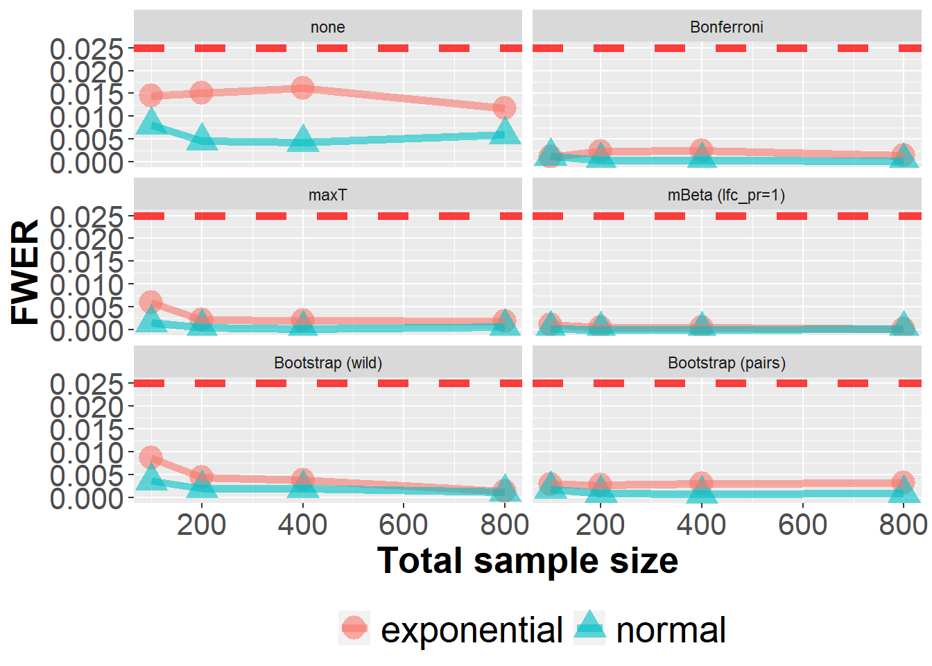

The next plot presents the same data slighty differently.

Code

data_sens_roc %>% 
  filter(n<1000) %>%
  filter(!(Adjustment %in% c("mBeta (lfc_pr=0.5)", "mBeta (lfc_pr=0)"))) %>% 
  group_by(Adjustment, n, prev, m, dist) %>%
  summarize(nsim=n(), rr = mean(`0` > 0)) %>%
  ggplot(aes(n, rr, col=Adjustment, fill=Adjustment, pch=Adjustment))+
  geom_point(size=6, alpha=0.6) +
  geom_line(size=2, alpha=0.6) +
  xlab("Total sample size") +
  ylab("FWER") +
  geom_hline(yintercept=0.025, col="red", lwd=2, lty=2, alpha=0.75) +
  owntheme +
  facet_wrap(~ dist, ncol=1)

`summarise()` has grouped output by 'Adjustment', 'n', 'prev', 'm'. You can
override using the `.groups` argument.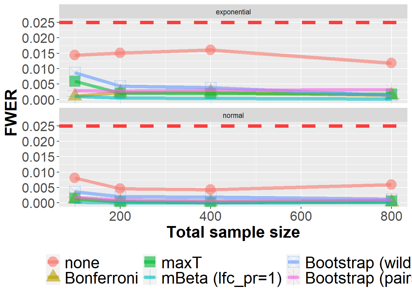

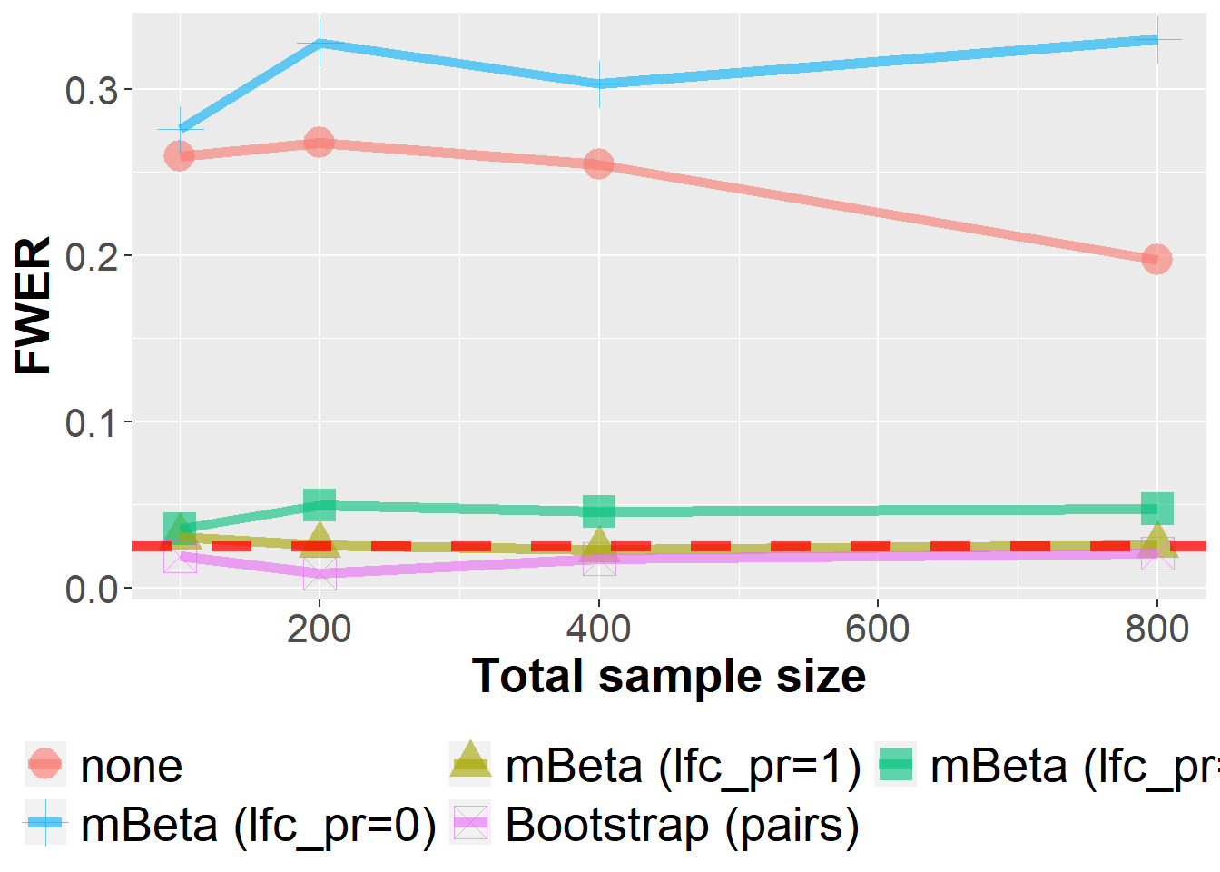
2.3.2 Prior influence of mbeta adjustment

The mBeta adjustment is a heuristic approach which builds on a Bayesian multivariate Beta-Binomial model. In this sensitivity analysis, the influence of the “lfc_pr’ hyperparameter is investigated. It lies in the unit interval and controls if the prior distribution is solely a least-favorable parameter configuration (lfc_pr=1, default), a mixture distribution (lfc_pr=0.5) or solely a uniform distribution (lfc_pr=0). As we can see below, this parameter has a noticeable influence on operating characteristics as the FWER.

Code

data_sens_roc %>% 
  filter(n<1000, dist=="normal") %>%
  filter(Adjustment %in% c("none", "mBeta (lfc_pr=1)", "mBeta (lfc_pr=0.5)", "mBeta (lfc_pr=0)", "Bootstrap (pairs)")) %>% 
  group_by(Adjustment, n, prev, m, dist) %>%
  summarize(nsim=n(), rr = mean(`0` > 0)) %>%
  ggplot(aes(n, rr, col=Adjustment, fill=Adjustment, pch=Adjustment))+
  geom_point(size=6, alpha=0.6) +
  geom_line(size=2, alpha=0.6) +
  xlab("Total sample size") +
  ylab("FWER") +
  geom_hline(yintercept=0.025, col="red", lwd=2, lty=2, alpha=0.75) +
  owntheme + 
  guides(fill=guide_legend(nrow=2, byrow=TRUE),
         col=guide_legend(nrow=2, byrow=TRUE),
         pch=guide_legend(nrow=2, byrow=TRUE))

`summarise()` has grouped output by 'Adjustment', 'n', 'prev', 'm'. You can
override using the `.groups` argument.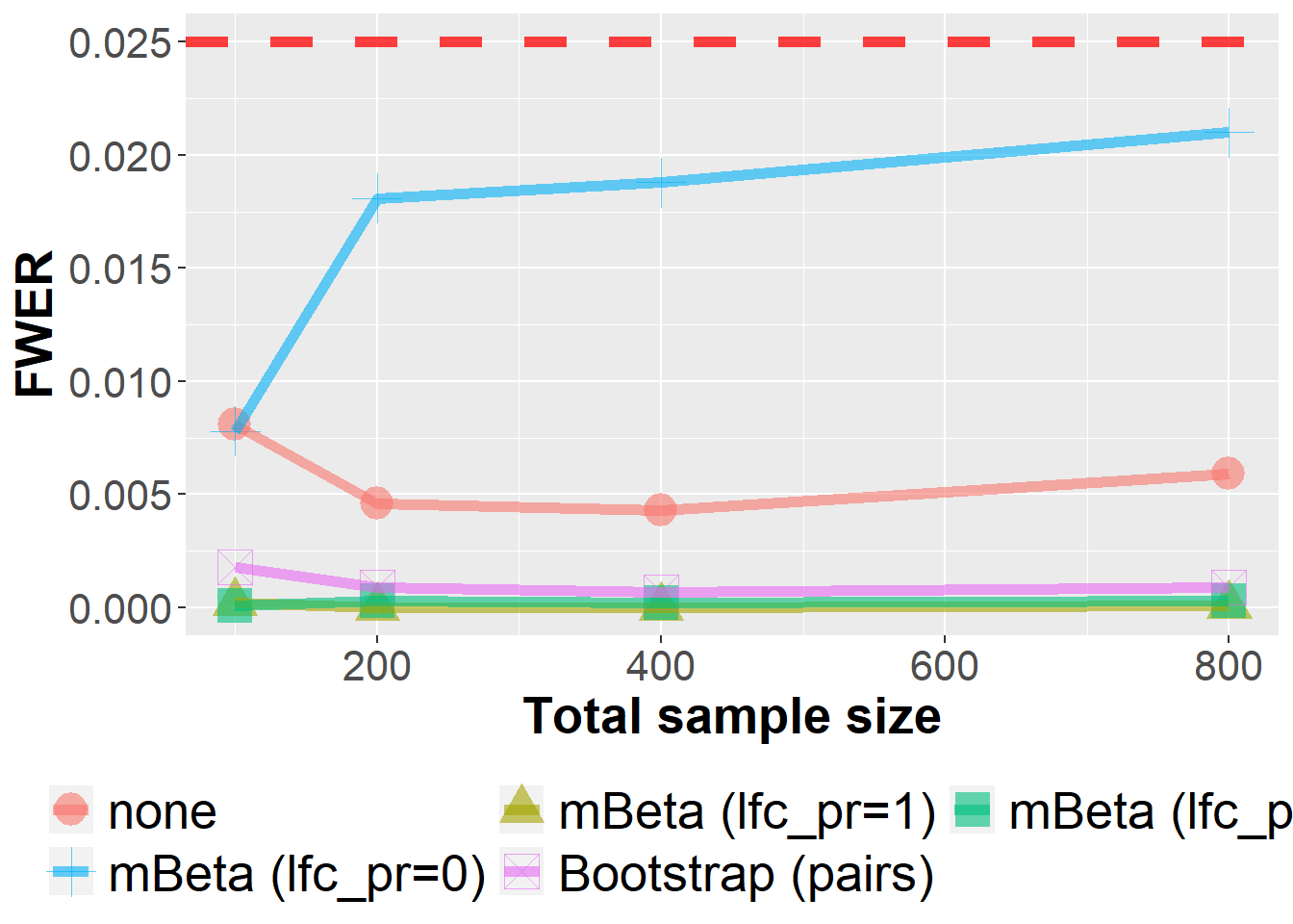

Code

data_sens_lfc %>% 
  filter(n<1000, se==0.8) %>%
  filter(Adjustment %in% c("none", "mBeta (lfc_pr=1)", "mBeta (lfc_pr=0.5)", "mBeta (lfc_pr=0)", "Bootstrap (pairs)")) %>% 
  group_by(Adjustment, n, prev, m, se) %>%
  summarize(nsim=n(), rr = mean(`0` > 0)) %>%
  ggplot(aes(n, rr, col=Adjustment, fill=Adjustment, pch=Adjustment))+
  geom_point(size=6, alpha=0.6) +
  geom_line(size=2, alpha=0.6) +
  xlab("Total sample size") +
  ylab("FWER") +
  geom_hline(yintercept=0.025, col="red", lwd=2, lty=2, alpha=0.75) +
  owntheme + 
  guides(fill=guide_legend(nrow=2, byrow=TRUE),
         col=guide_legend(nrow=2, byrow=TRUE),
         pch=guide_legend(nrow=2, byrow=TRUE))

`summarise()` has grouped output by 'Adjustment', 'n', 'prev', 'm'. You can
override using the `.groups` argument.